Project 3 / Camera Calibration and Fundamental Matrix Estimation with RANSAC
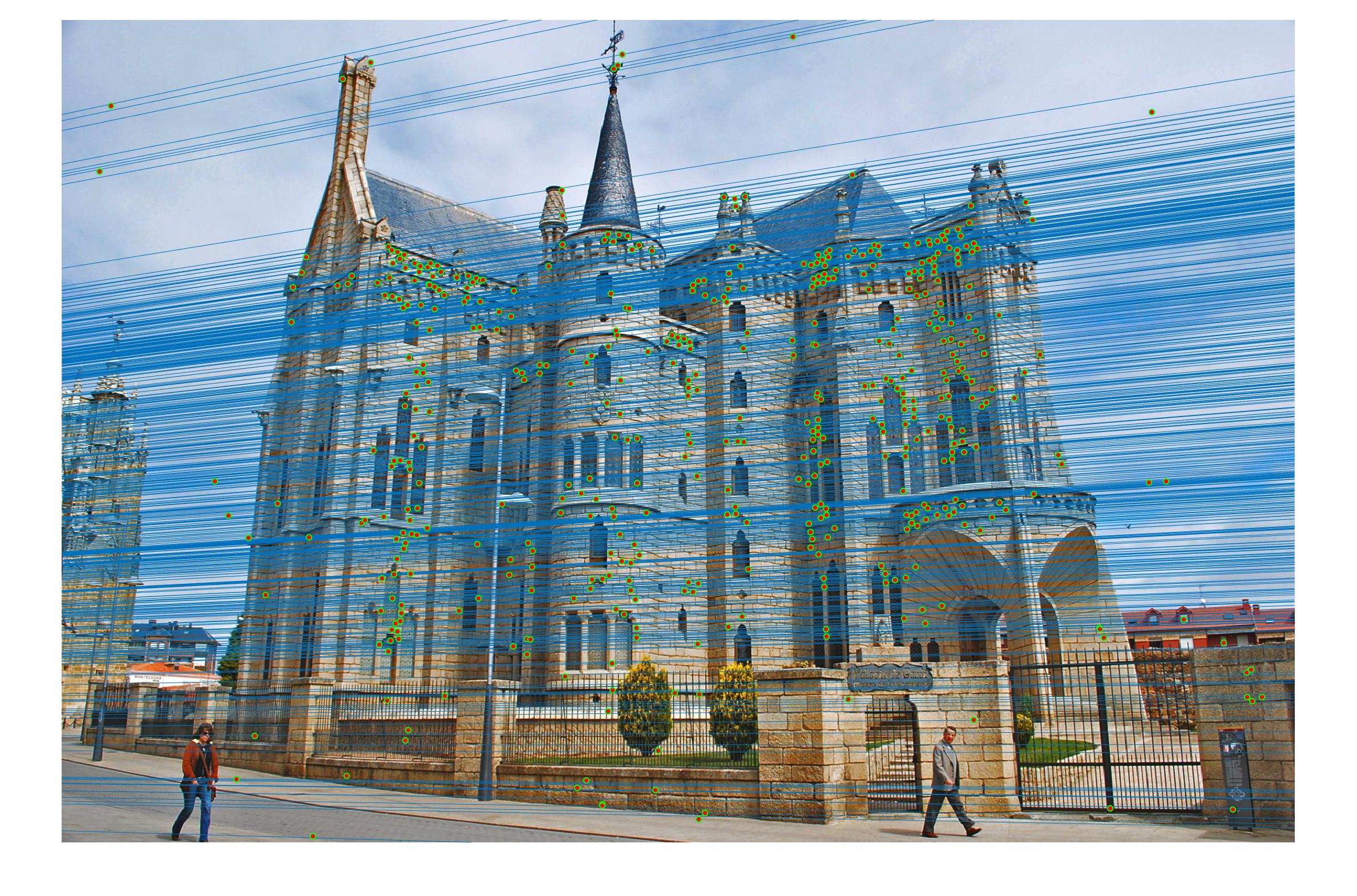
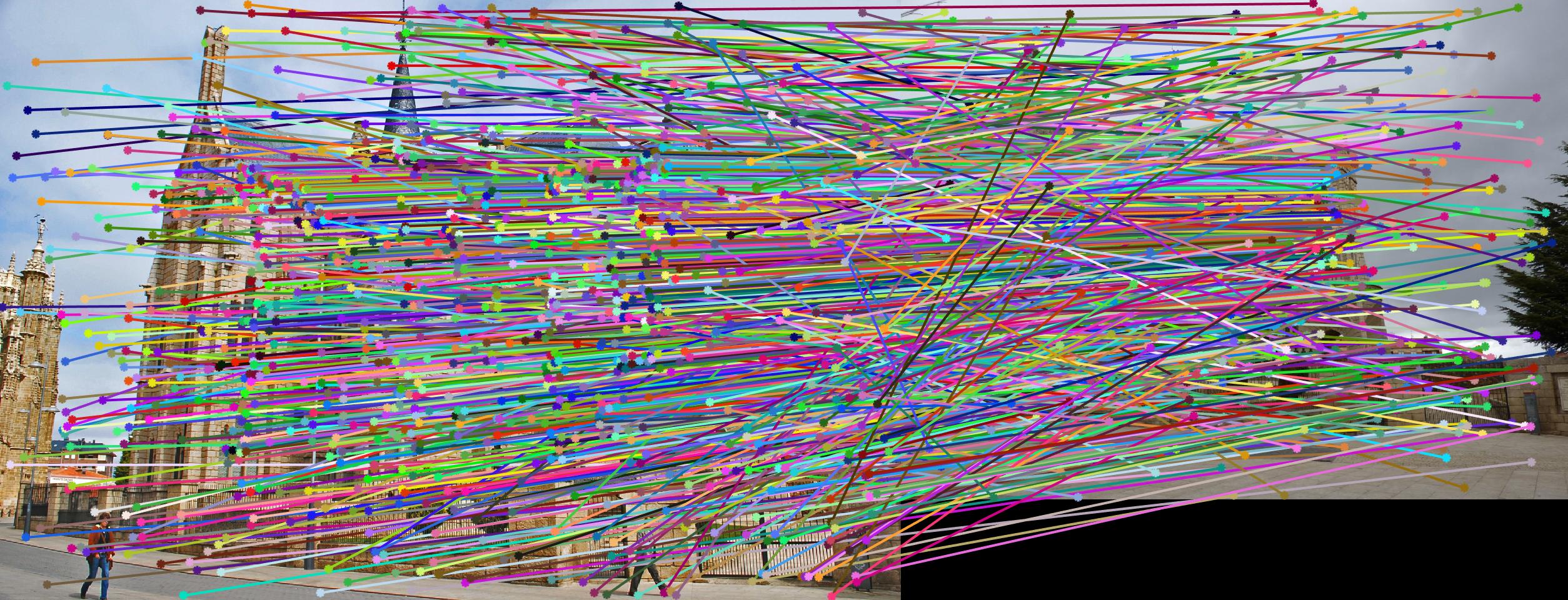
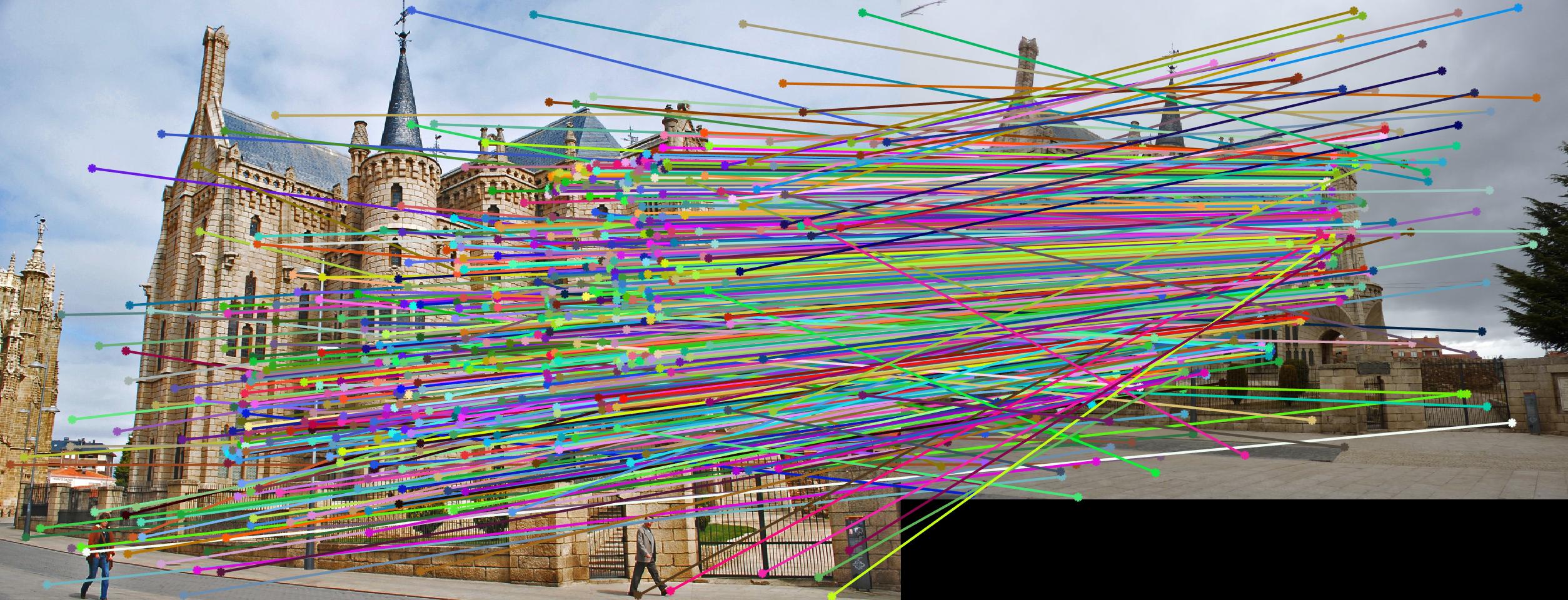
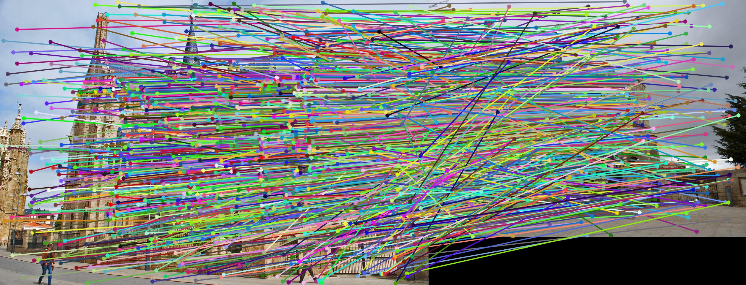
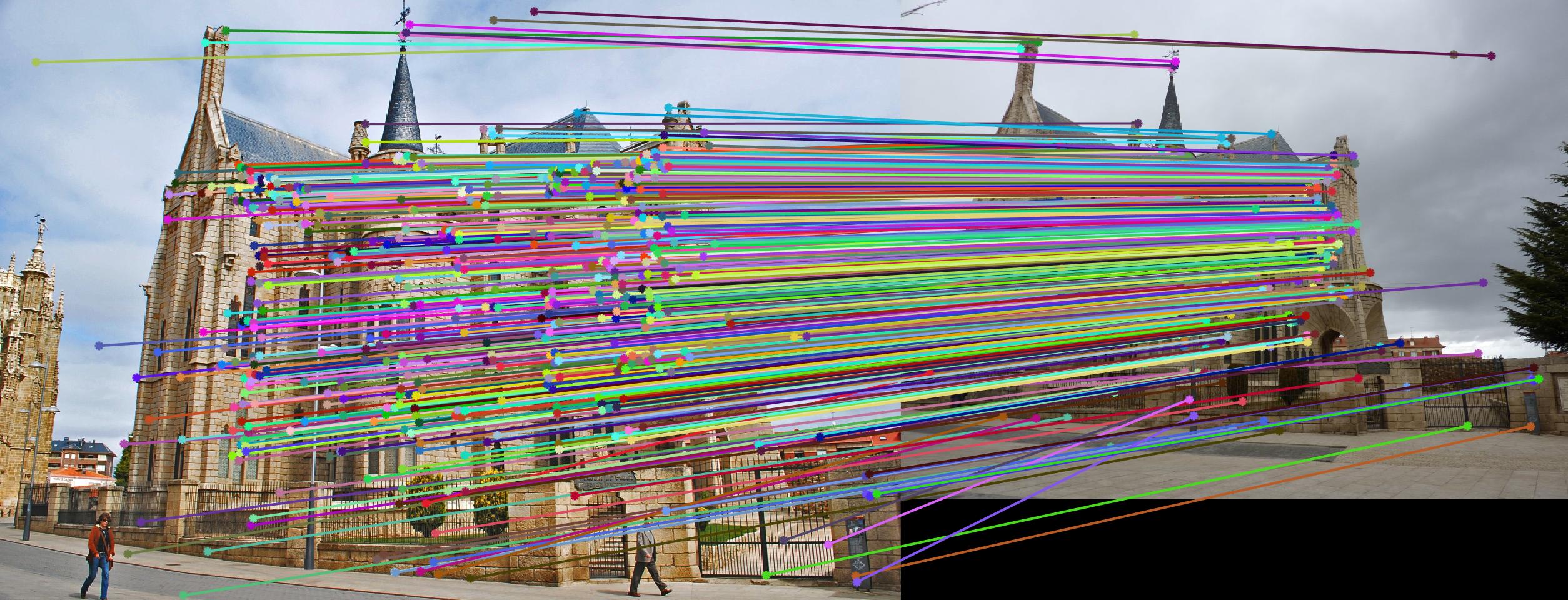
Fig 1. RANSAC on Gaudi images: 1500 iterations, inlier threshold = 0.03 gives 505 matching points with epipole out scope.
In this project I developed algorithms to perform camera calibration by estimating the projection matrix as well as estimating the fundamental matrix between pairs of (stereo) images with the help of RANSAC to prune spurious matching points. As a three stage process, the project was completed by first estimating the projection matrix by formulating a linear system of known 2D image coordinates matched with 3D locations in worldview. I then solved for the projection matrix M using the 2nd method found in lecture 14 slides. Because I fixed the scale before doing a linear least squares regression by always appending 1 to the end of homogeneous column vectors and the last entry of M, we know that the estimated projection matrix would not be all zeros and should be invariant to differences in scale. To verify my results, the resulting matrix found below is indeed a scaled version of the reference solution. 
= scaleProj - 1/0.5968 = 1.6756 * 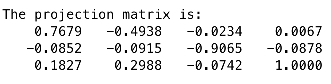
I was able to verify my calculated projection matrix to be correct by looking at the total residual value which came out to be 0.0445 with the normalized image & world coordinates. When switching to unnormalized coordinates, I observed a slight increase in total residual value to 15.6217, which is expected as the reason we normalize is to make the least squares solution more robust, and this verifies that preprocessed normalization worked.
Once I found the projection matrix, I was able to compute the camera center by breaking matrix M into matrix K of intrinsic parameters and matrix [R | T] of extrinsic parameters. Instead of manually decomposing M however, in class we've learned a trick to compute just the camera center coordinates by C = -Q-1m4. By some matrix slicing and manipulation, I obtained an estimated camera location of <-1.5126, -2.3517, 0.2827>. Which, as expected, is once again really close to the reference solution of CnormA = < -1.5125, -2.3515, 0.2826 >.
Part II. Estimating the Fundamental Matrix
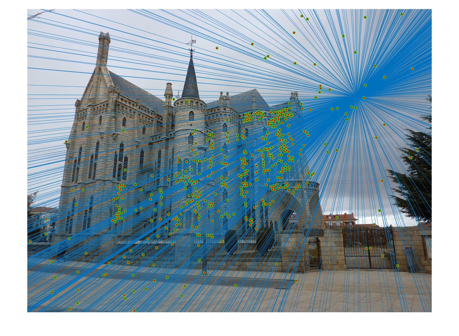
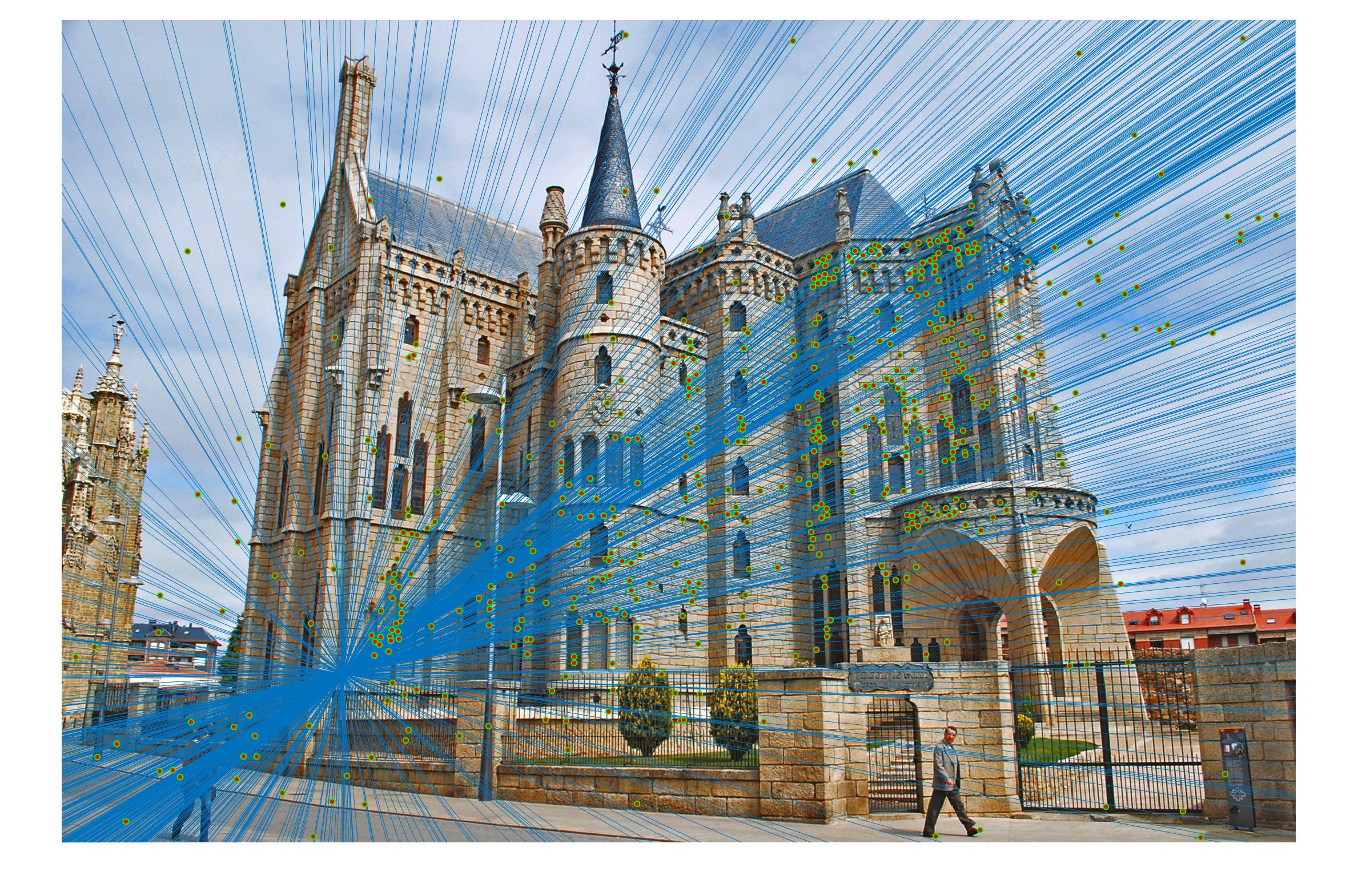
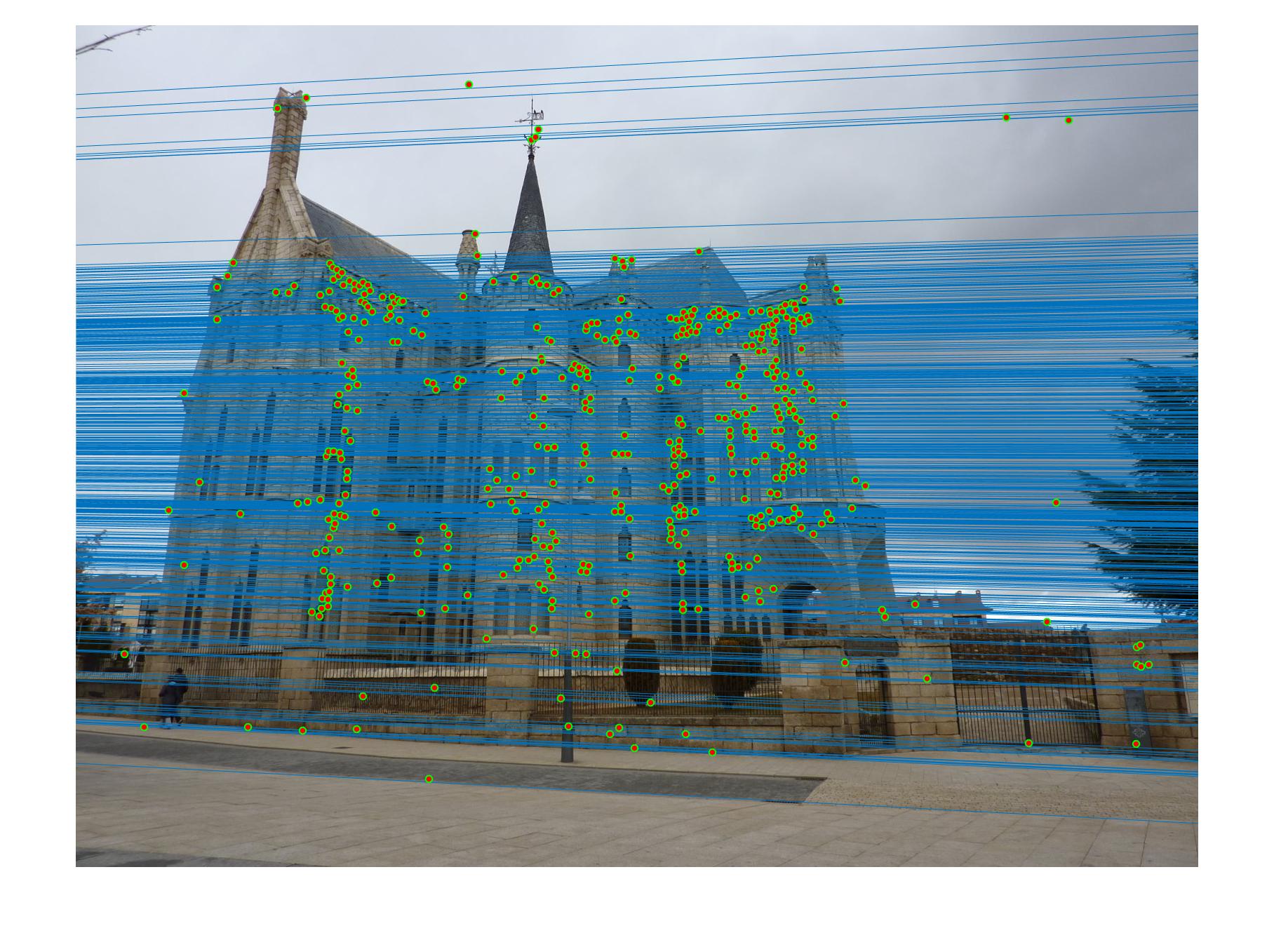
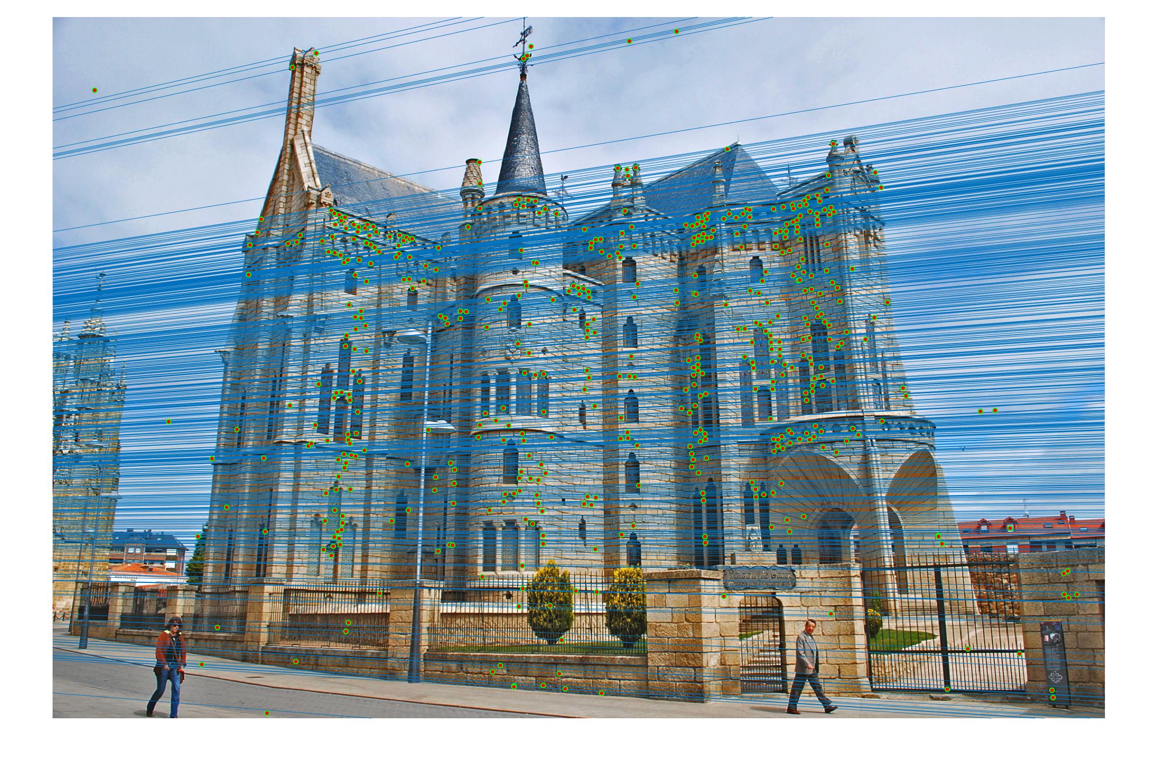
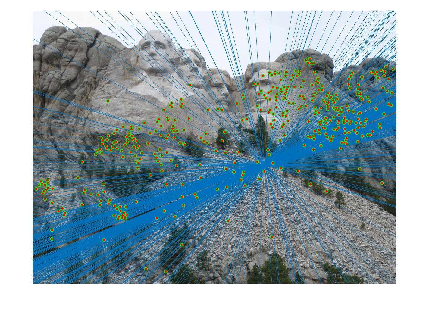
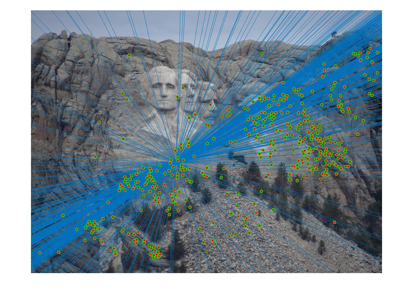
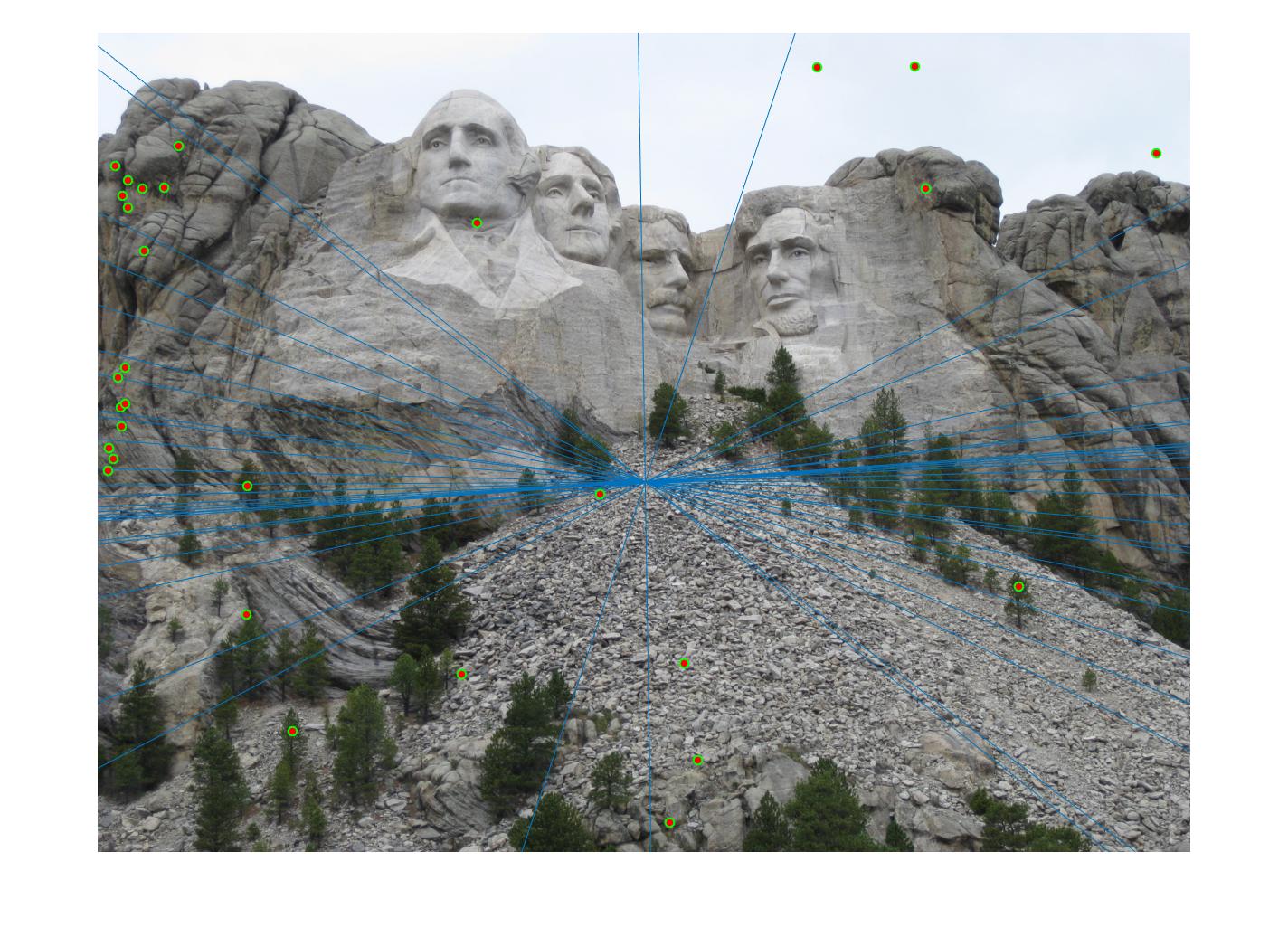
The second stage in the pipeline is to estimate the fundamental matrix using epipolar geometry of the interest points found in the two images. For the sake of performance, SIFT interests points are computed by the VLFeat library functions in this project. Using the fundamental matrix definition provided I was able to construct a linear system of equations that had more variables than the number of equations. Being an overdetermined system it can have an infinite number of solutions so to ensure that we get a non-zero fundamental matrix I had to fix the last element of matrices to 1 to reduce the dimensionality and solve by the linear least squares method suggested in lecture 13 slides. Much like in part 1, many matrix manipulation operators were used to streamline for performance and minimize for loops. Through SVD analysis I was able to drop the smallest singular value of the fundamental matrix so epipolar lines will now instersect at a common point called the epipole. To verify that our fundamental matrix estimation is sensible and useful, see below that epipolar lines are indeed crossing through the corresponding ground truth points in the other image. There is one caveat to note, however, that this fundamental matrix is not the true "correct" fundamental matrix that describes the two perpectives in real life due to limitations in Field of View of a photograph and other factors. Nevertheless in image pairs where planes are strictly defined like the one we see below, the estimated fundamental matrix is does a pretty good job constraining the search space for point correspondences.
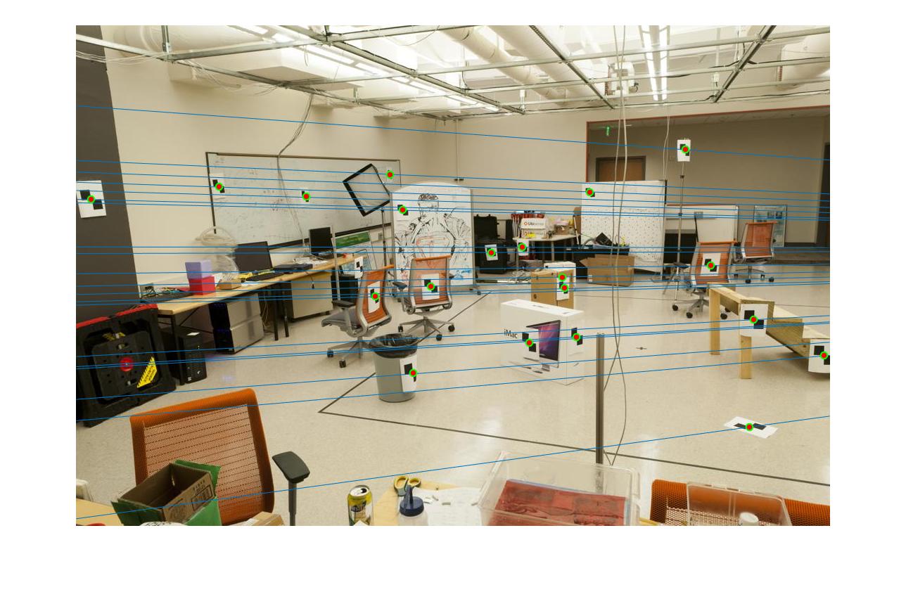
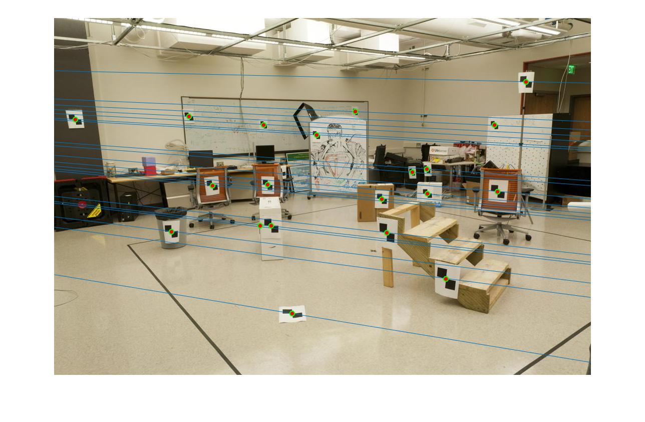
Fig 2. all of the epipolar lines cross through the corresponding point in the other image, vice versa
Estimating of Fundamental matrix for pic_a.jpg and pic_b.jpg
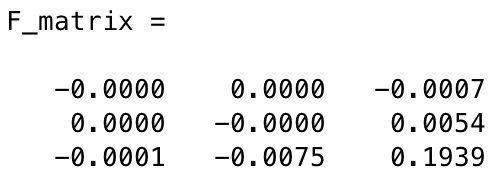
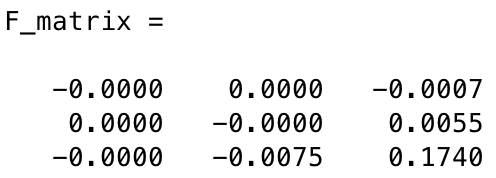
Fig 3. (left) Estimated fundamental matrix by default (right) Estimated fundamental matrix from points with noise (normalization workaround)
After

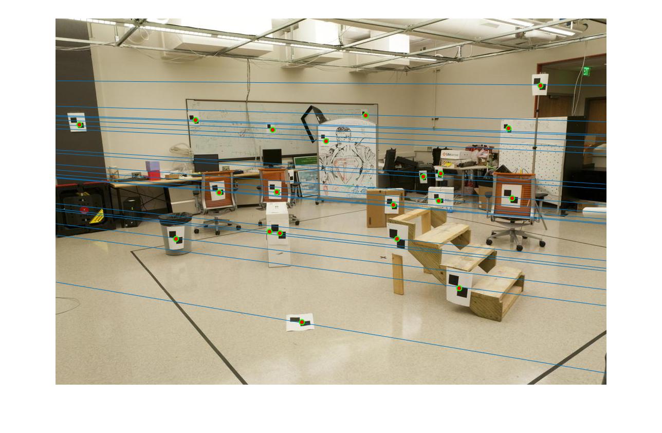
Fig 3b. even with added noise and a different fundamental matrix, all of the epipolar lines still cross through the corresponding point in the other image
Part III. Reject spurious matchings with RANSAC
The last stage in the pipeline is to refine the fundamental matrix we found from Part II. As the fundamental matrix could be ill-conditioned and influenced by scale imbalances between the x- and y-axes, the fundamental matrix can be unrepresentative of the transformation from a feature point to its corresponding epipolar line in the other image. This bias may be augmented especially when we have a large number of SIFT keypoints returned to search from (comparison statistics shown at the end). To reject spurious and minimize mismatches, we use the RANSAC algorithm to randomly sample 8 points of all keypoints to generate a different fundamental matrix every iteration. We then find how many inliers are within a threshold of agreement with the fundamental matrix. To determine this level of agreement, we define a distance metric as product x'Fx for a pair of point correspondence (x',x) and fundamental matrix F. Because we know in theory that a proper fundamental matrix of true epipolar points should yield x'Fx = 0, we want to minimize x'Fx for a randomly sampled F. Upon every iteration, we update the maximum number of inliers counted as well as its corresponding fundamental matrix. At the end of the algorithm, we denote this maximum-inlier Fundamental matrix as the "Best Fundamental Matrix" found.
In our RANSAC algorithm, two parameters are adjustable: the number of iterations, and the inlier threshold. The following is my RANSAC pseudocode:
% 1) randomly sample 8 pairs of point correspondences using MATLAB's randsample() with range = # input keypoints (x', x)
% 2) pass in the point correspondences, stored as new vectors samp_a and samp_b, to our estimate_fundamental_matrix() implementation from Part 2.
% 3) iterate all the input keypoints (x', x) and compute x'Fx, where if x'Fx < some threshold we increment the number of inliers seen.
% 4) update the highest number of inliers seen as well as the fundamental matrix with the most inliers. Goto next iteration.
After extensive trial and error with # iterations ranging from 20 - 30,000 and inlier threshold 0.5 down to 0.01, I found that the best performing set of
parameters that yielded the most accurate, correct and prolific keypoint correspondences is threshold = 0.03 and #iterations = 1500. This pair of parameters worked quite well for all images tested and is believed to yield strong results with a good balance between outlier minimization and computation efficiency for the general case compared to other parameter combinations like
[{threshold=0.05, #iterations=1000}, {threshold=0.01}, #iteration=30000}]. Below are some illustrations of improvement.
=>
=>

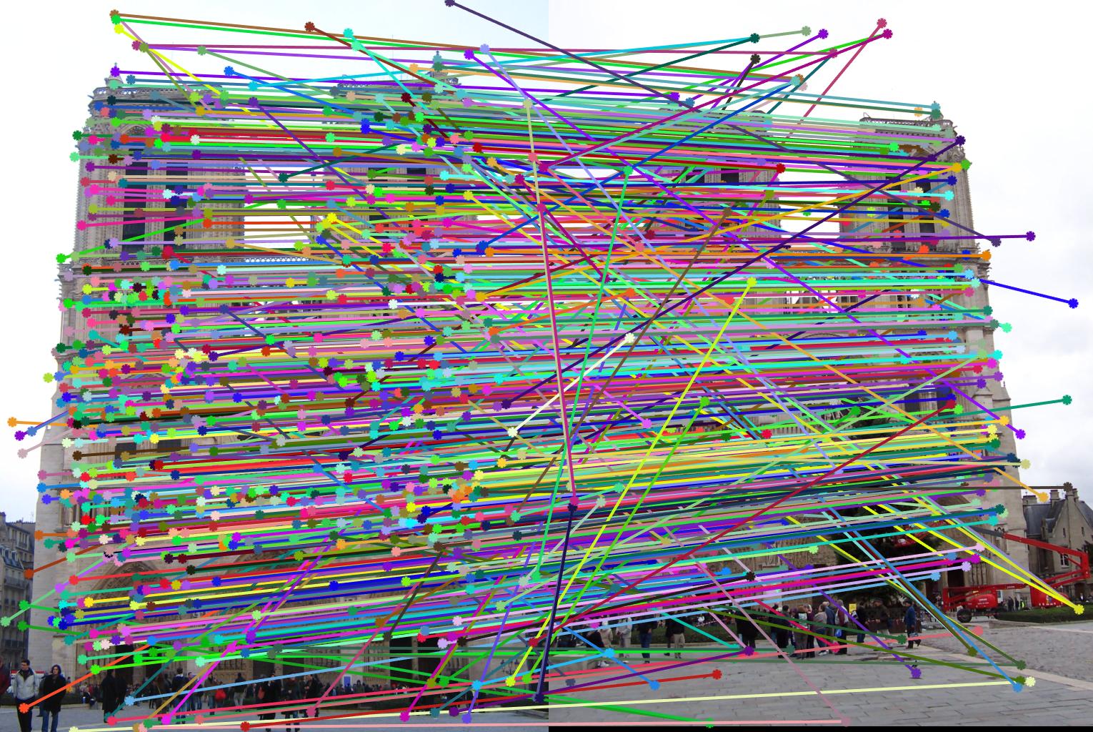
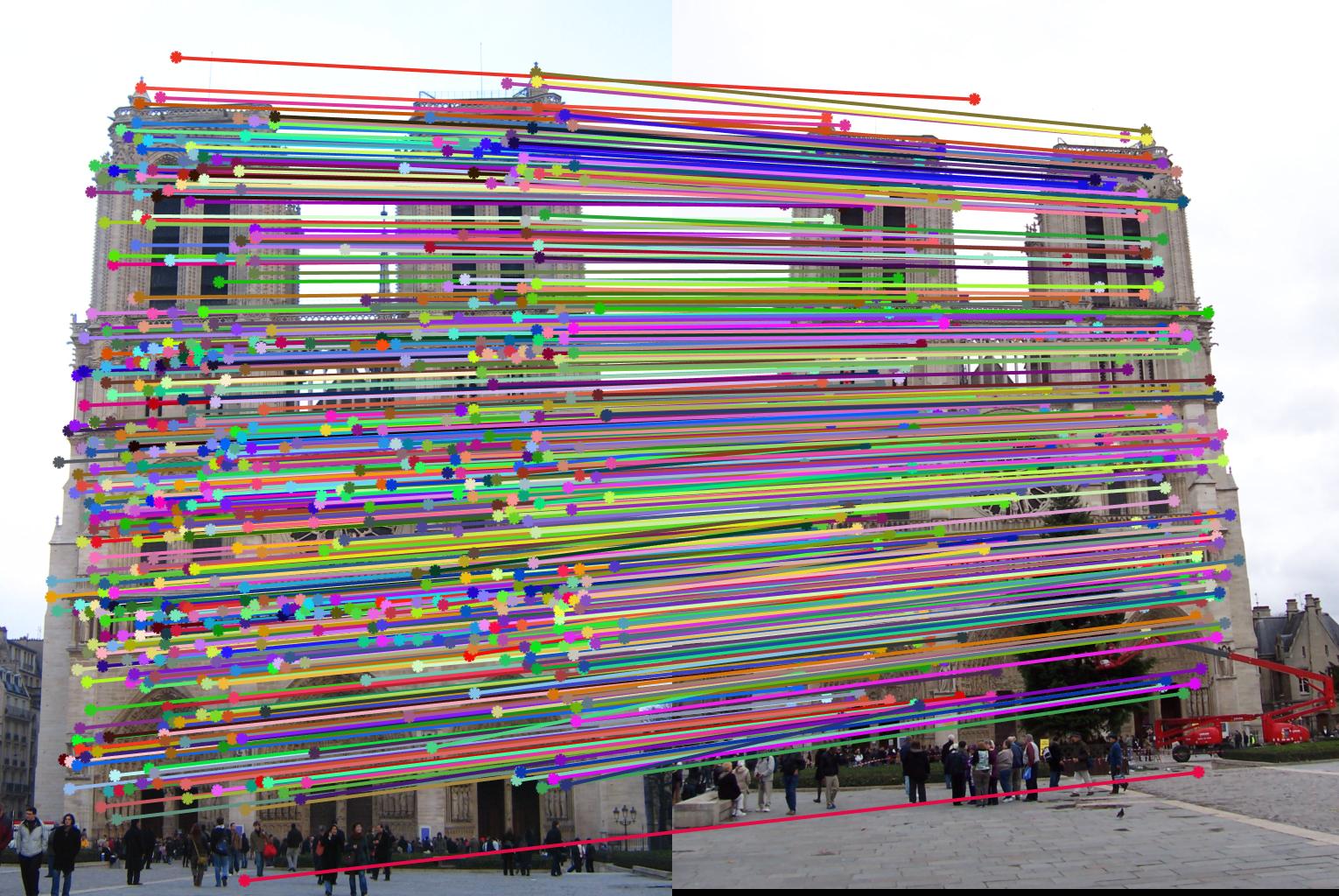
Fig 4. improvement progression: (left) part 3 unimplemented --> (middle) RANSAC, bad parameters --> (right) RANSAC, threshold=0.03, #iterations=1500
Extra Credit
Even with RANSAC and the "best" pair of parameters determined, some difficult images like the Gaudi pair still showed many incorrect correspondences. This is due to the fact that the fundamental matrix that is estimated is "wrong" (as in it implies a relationship between the cameras that must be wrong, e.g. an epipole in the center of one image when the cameras actually have a large translation parallel to the image plane) - project description. The estimated fundamental matrix can be off because of poor numerical conditioning of the image coordinates used to determine our fundamental matrix. That is, of the keypoints returned by SIFT, some of their x and y coordinates can vary signficantly enough that the fundamental matrix becomes ill-conditioned. To address this problem, I proceeded to normalize keypoint coordinates through a linear transformation described by a combination of scaling and translation. That is, we 'normalize' so that the camera center is at the origin, and the points are at most a standard deviation away from the mean (origin). Implemented in estimate_fundamental_matrix() is the following add-on normalization procedure.
% Normalized 8-point algorithm: preprocessing

% stdA = std2(Points_a);	% use this if we wanted both scale s1, s2 to be consistent
stdAx = std(Points_a(:,1));	% standard deviation w.r.t. x-axis
stdAy = std(Points_a(:,2));	% standard deviation w.r.t. y-axis
scaleA = [1/stdAx 0 0; 0 1/stdAy 0; 0 0 1];

% stdB = std2(Points_b);	% use this if we wanted both scale s1, s2 to be consistent
stdBx = std(Points_b(:,1));	% standard deviation w.r.t. x-axis
stdBy = std(Points_b(:,2));	% standard deviation w.r.t. y-axis
scaleB = [1/stdBx 0 0; 0 1/stdBy 0; 0 0 1];

% Offset matrix: Mean of x and y coordinates
meanAx = mean(Points_a(:,1));
meanAy = mean(Points_a(:,2));
offsetA = [1 0 -meanAx; 0 1 -meanAy; 0 0 1];

meanBx = mean(Points_b(:,1));
meanBy = mean(Points_b(:,2));
offsetB = [1 0 -meanBx; 0 1 -meanBy; 0 0 1];

Ta = scaleA * offsetA;	% Translation and scale matrix for matched points in image_A
Tb = scaleB * offsetB;	% Translation and scale matrix for matched points in image_B

% -- 8-point algorithm with Ta * image_A points and Tb * image_B points -- %
Forig = Tb' * F * Ta;	% un-normalize fundamental matrix back to original units
Results of normalization
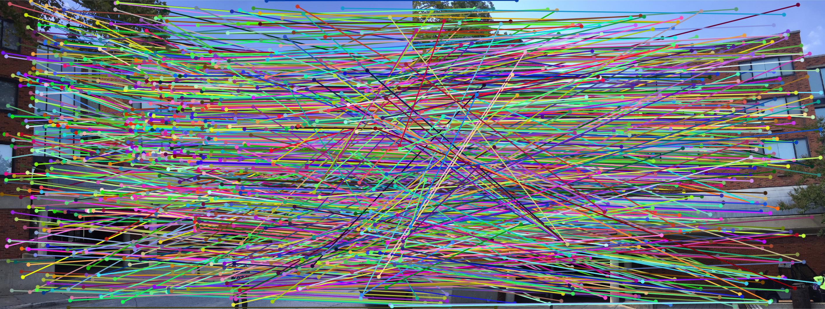
Gaudi - before:
Gaudi - after:
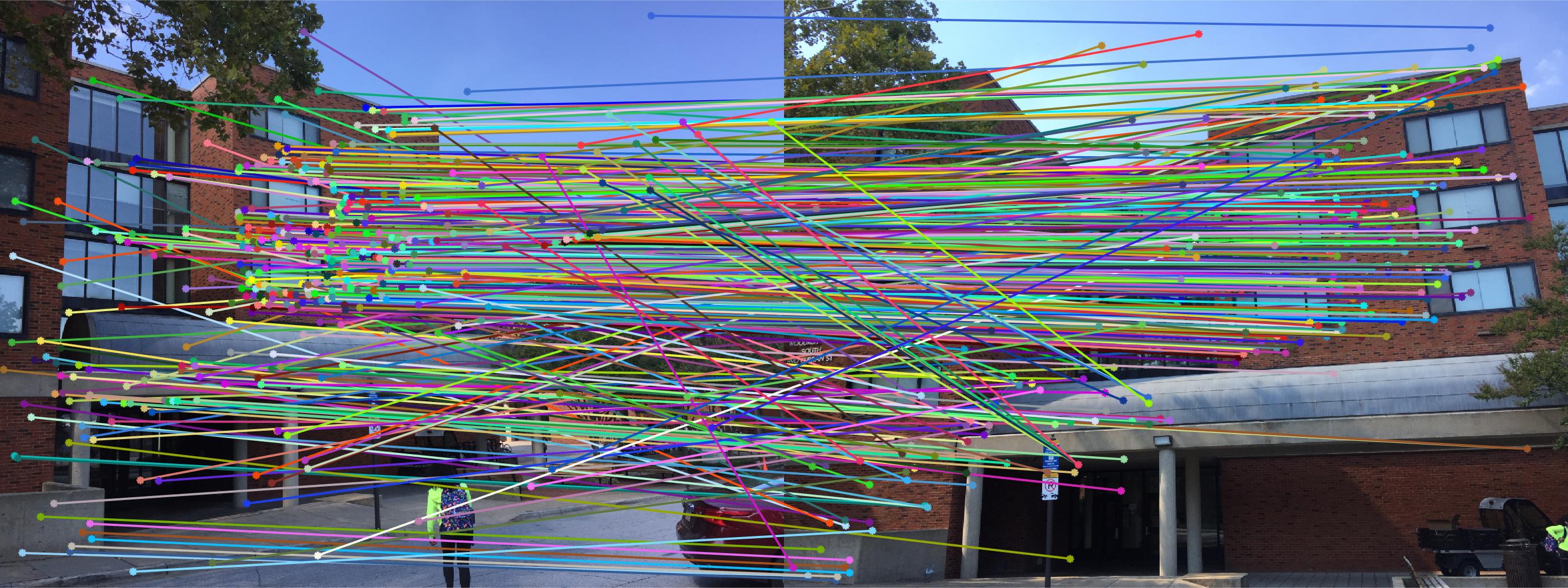
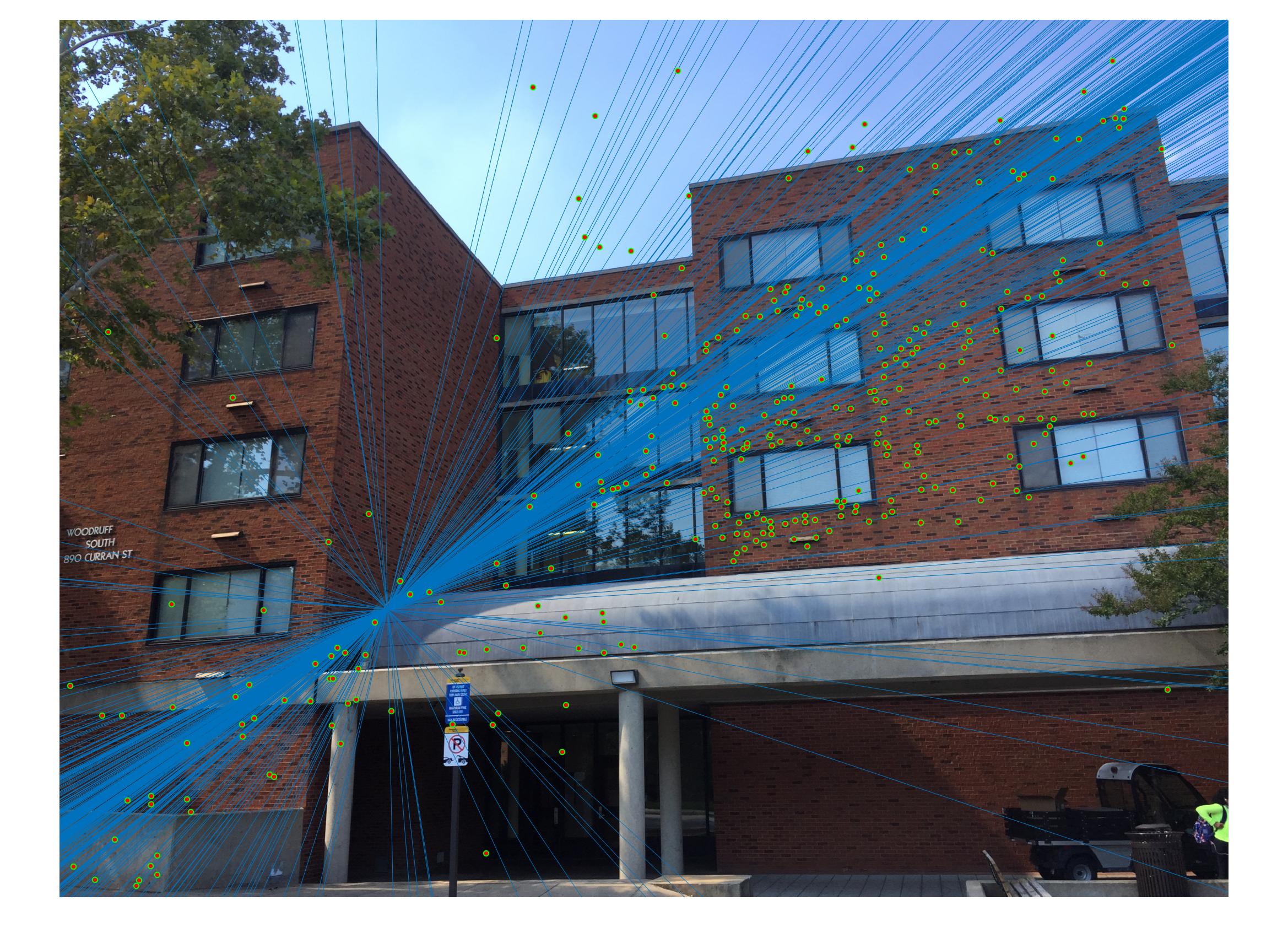
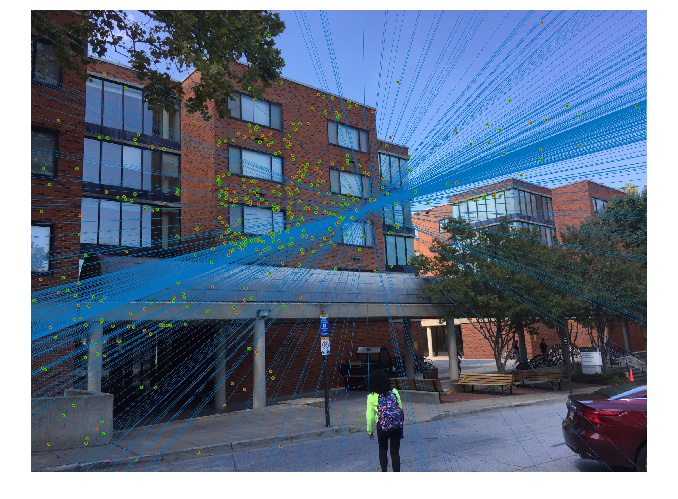
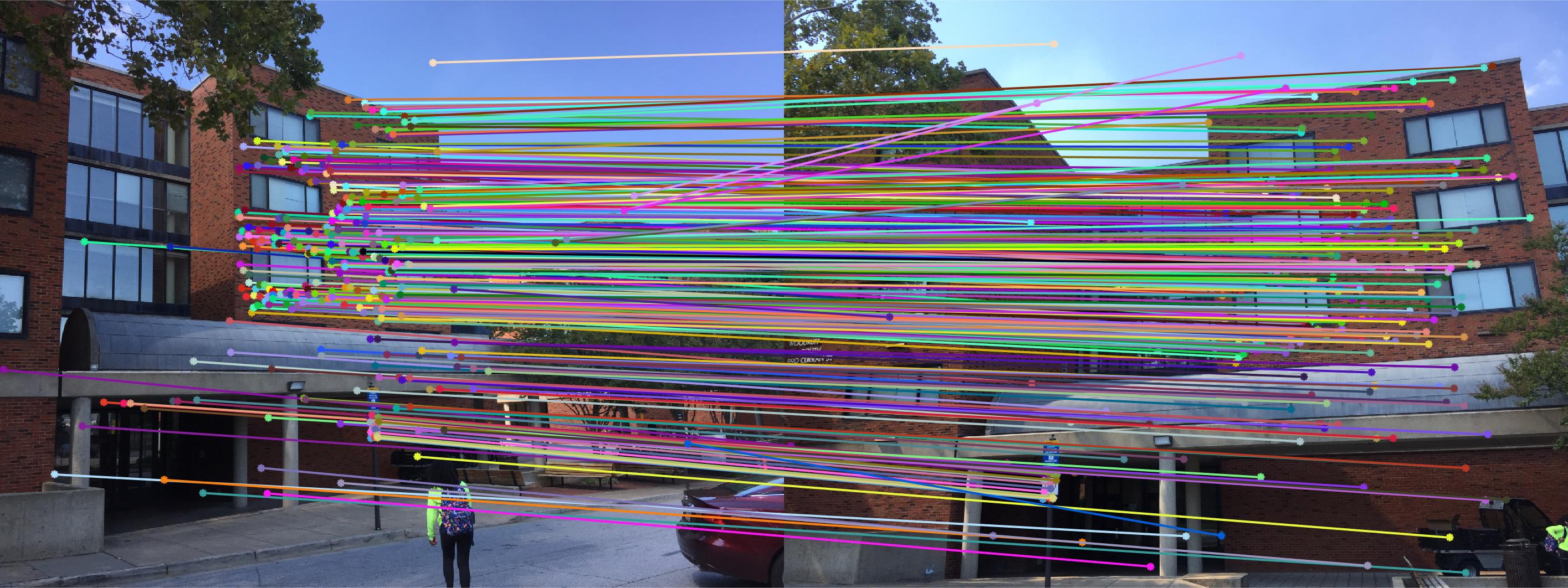
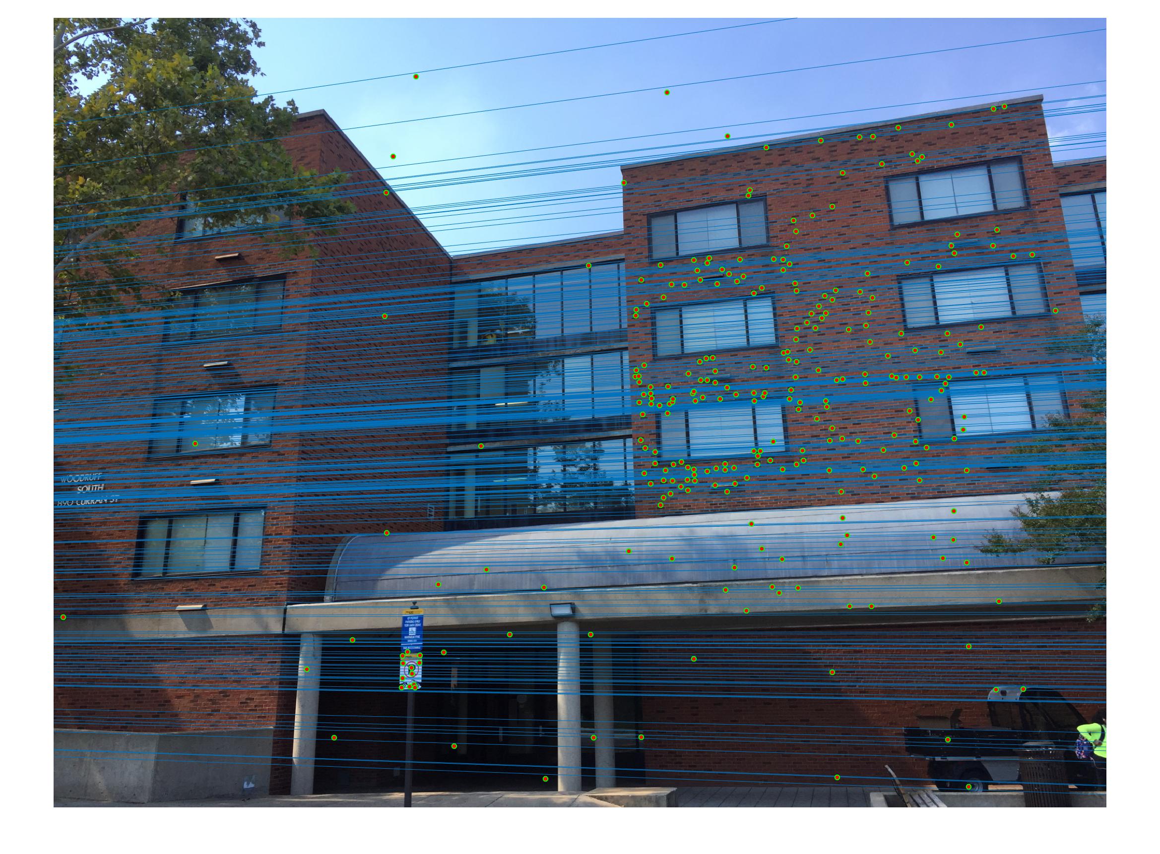
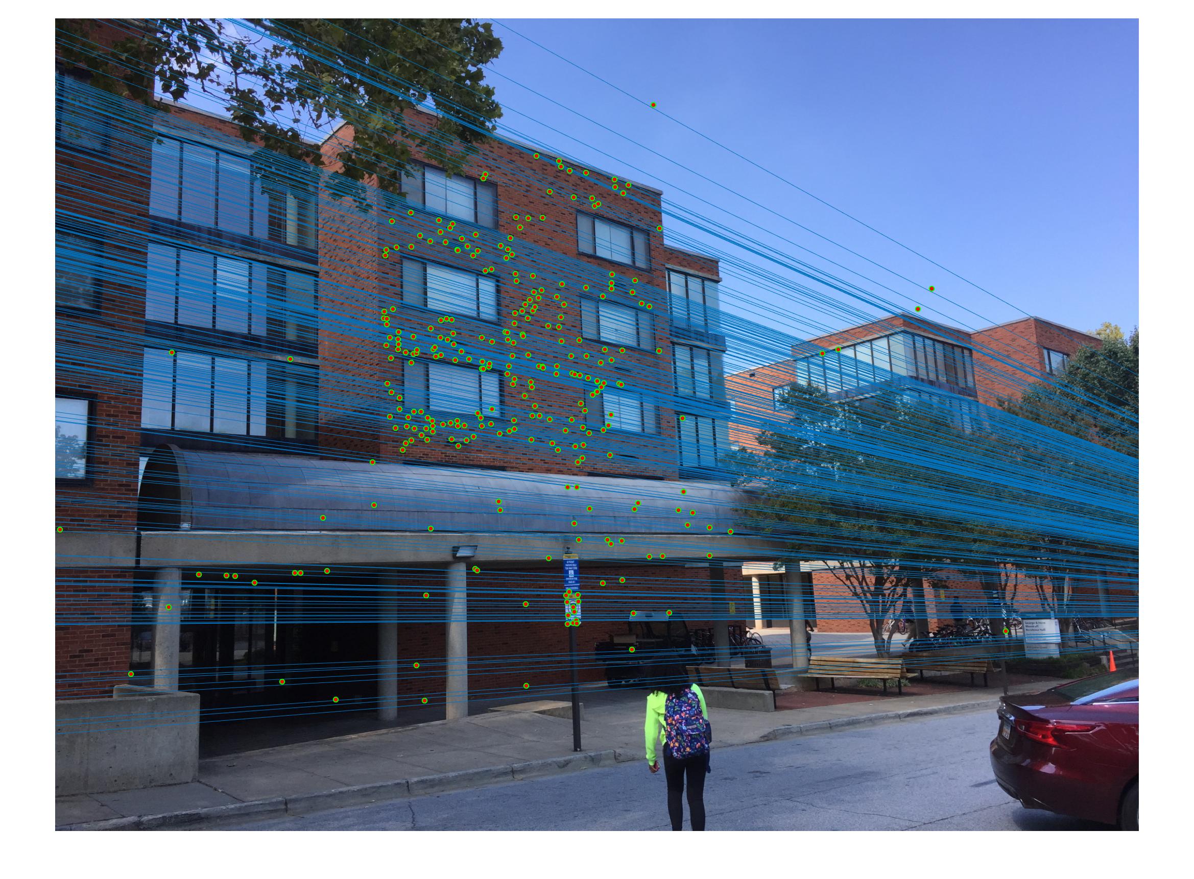
Woodruff - before:
Woodruff - after:
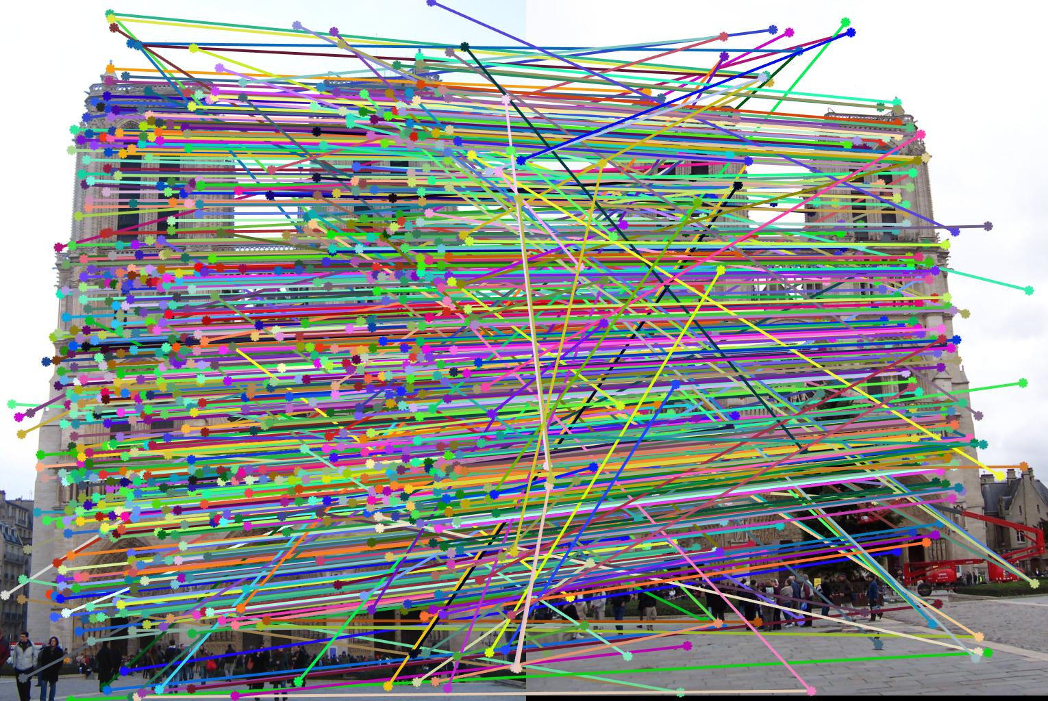
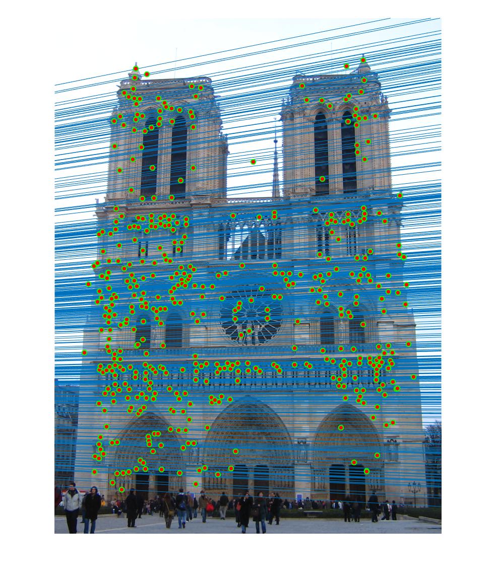
Notre Dame - before:
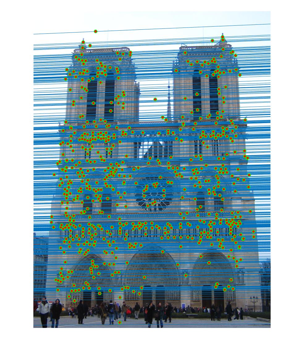
Notre Dame - after:
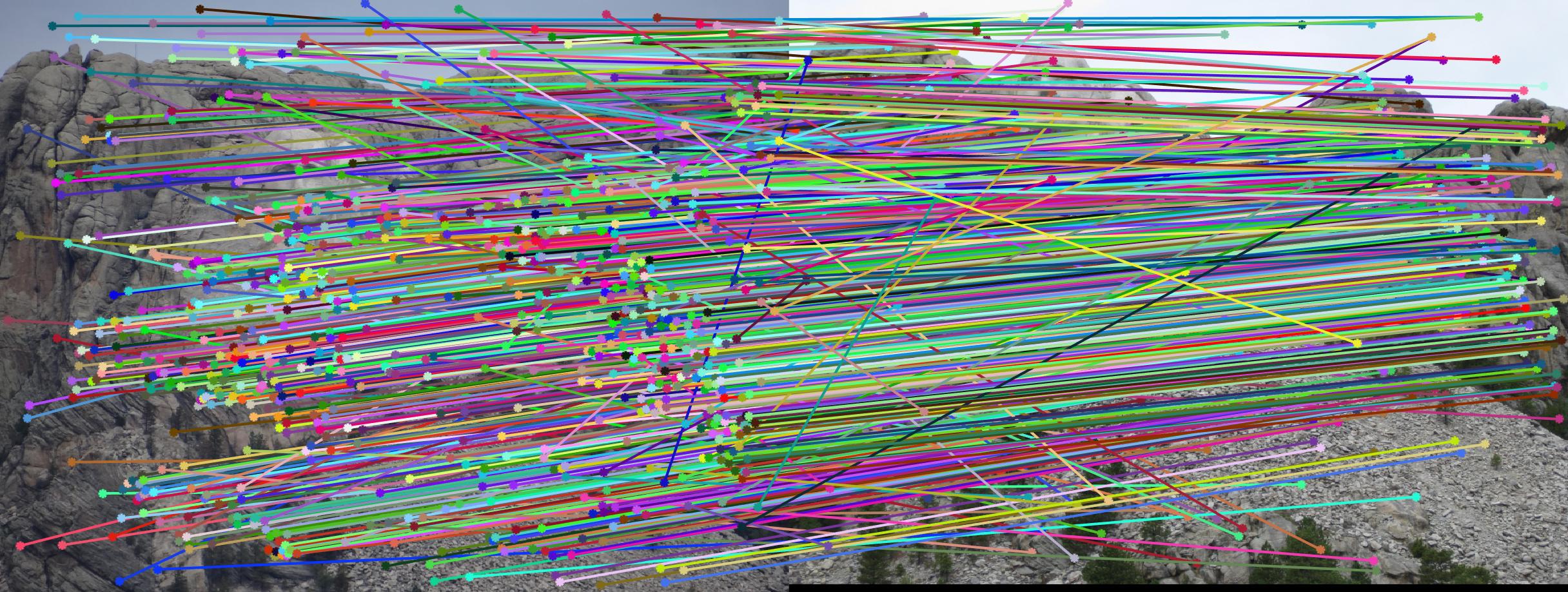
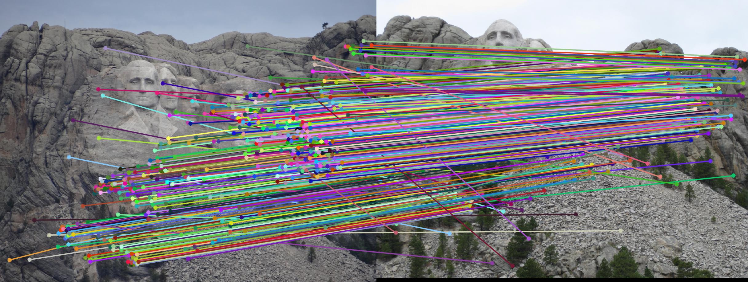
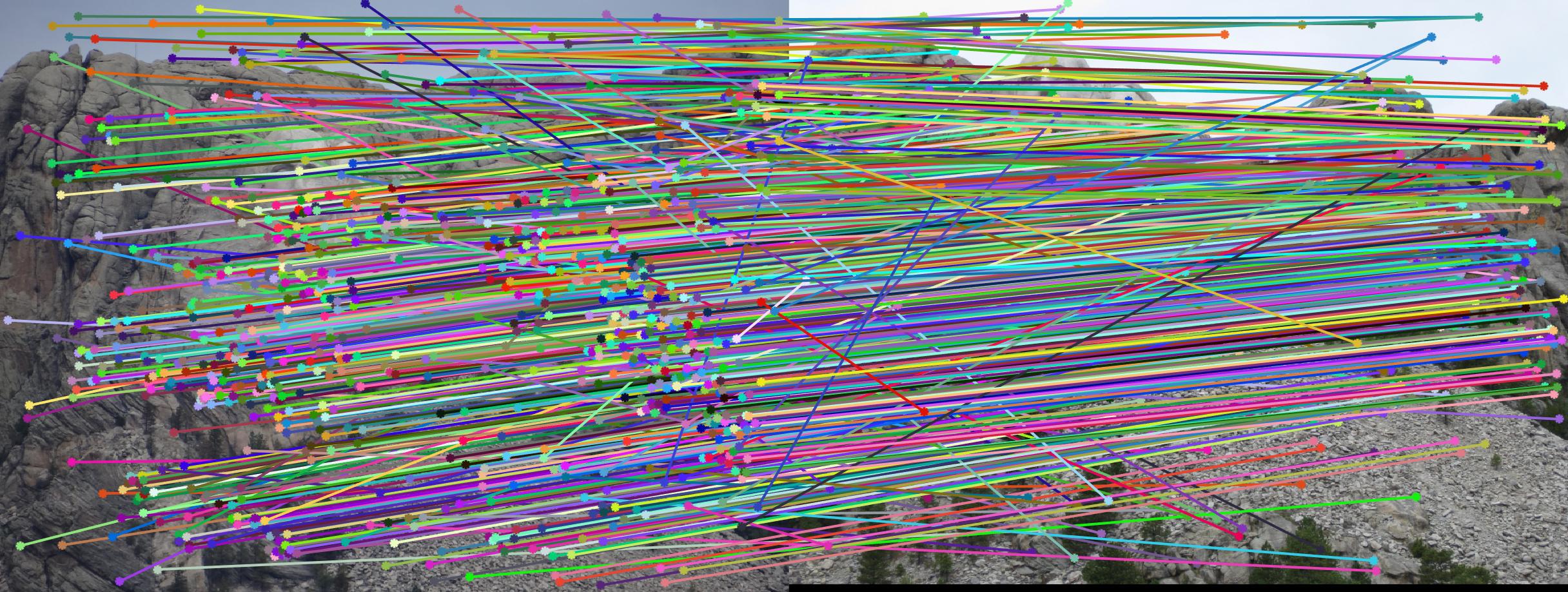
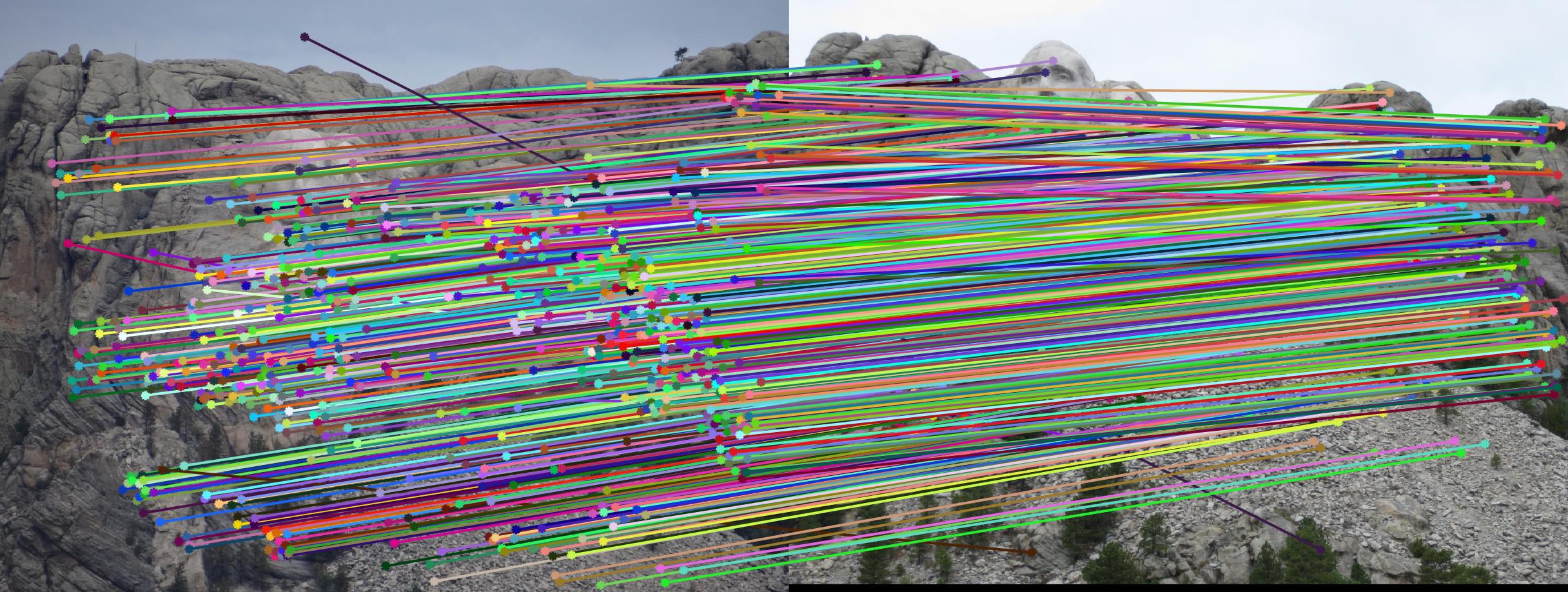
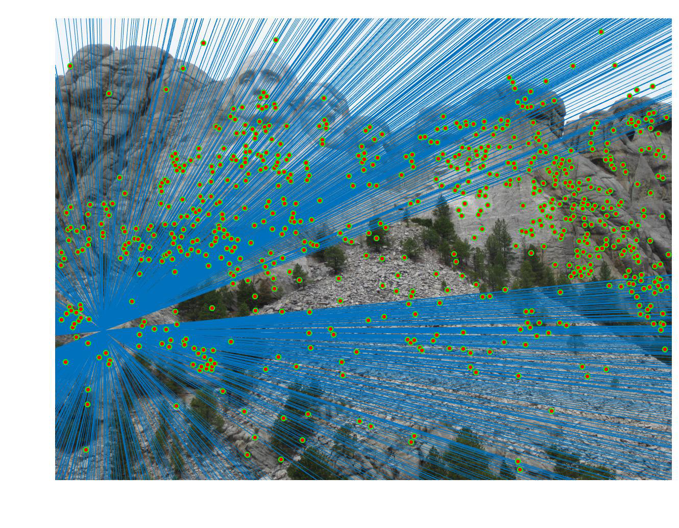
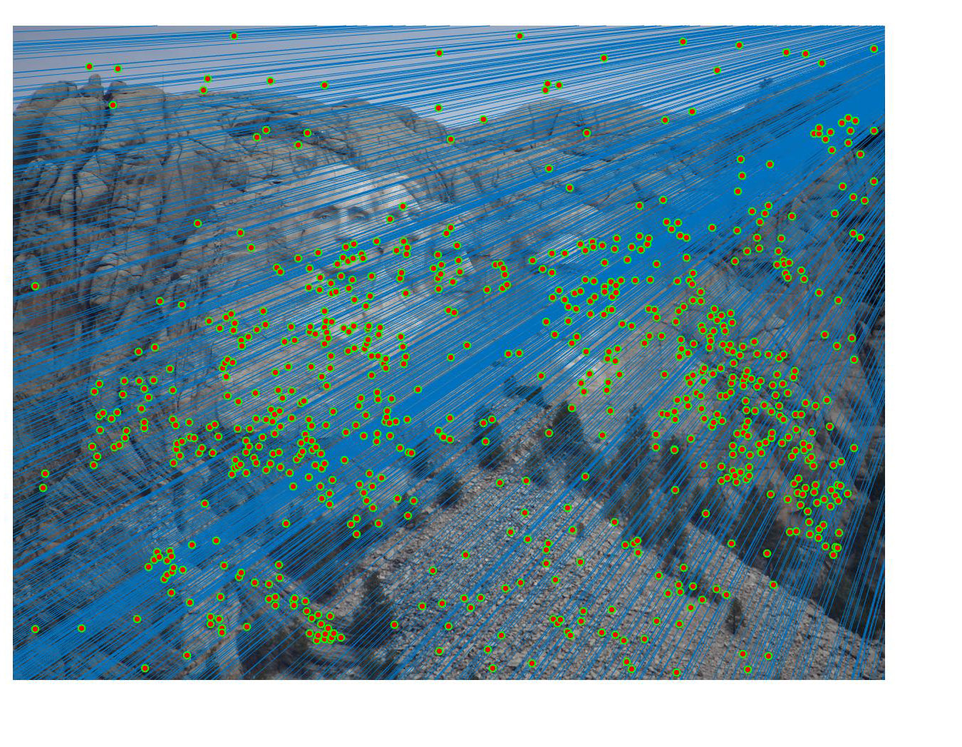
Mount Rushmore - before:
Mount Rushmore - after:
Growth Statistics comparison: unnormalized / normalized coordinates
Number of inlier correspondences vs. # of RANSAC iterations
| # iterations
| Rushmore: unnorm/norm (total 825) |
Gaudi: unnorm/norm (total 1062) |
ND: unnorm/norm (total 851) |
Woodruff: unnorm/norm (total 887) |
| 1500 |
501/668 | 498/505 | 491/680 | 400/291 |
| 3000 |
537/669 | 546/516 | 500/678 | 407/323 |
| 30000 |
559/669 | 553/517 | 499/683 | 417/335 |
Runtime vs. # of RANSAC iterations
| # iterations
| Rushmore: unnorm/normalized |
Gaudi: unnorm/normalized |
ND: unnorm/normalized |
Woodruff: unnorm/normalized |
| 1500 |
20.5s/25.88s | 32.45s/30.31s | 15.97s/24.06s | 30.55s/31.04s |
| 3000 |
27s/35.9s | 39.77s/38.9s | 24.13s/39.35s | 38.99s/53.23s |
| 30000 |
2min31.91s/3min47.48s | 3min22.13s/3min20.57s | 2min44.72s/3min47.2s | 2min57.22s/3min38.9s |
Trend analysis: It is not hard to spot an increasing trend down the columns for both tables as well as unnormalized vs. normalized points.
In terms of number of inlier keypoint correspondences found, we see that generally, the higher the number of iterations, the greater number of correspondences were found. Notre Dame pair is an exception to this (albeit figures all being very close), but notice from the results table that using normalized coordinates did not improve its correspondence results. Between unnormalized and normalized runs, it is usually the normalized coordinates that yields more correspondences. Again we have Woodruff dorm as an exception, likely due to the clearer-defined relationship between the cameras so the estimated fundamental matrix is less ambiguous even without any normalization.
In terms of computational runtime, a similar increasing trend follows as we go from low number of iterations to a high number. Due to the extra steps required to normalize and denormalize point coordinates/fundamental matrices, we also see that normalized runs take longer as expected.