Project 6 / Deep Learning
In this final project, we explore the use of Deep Convolutional Neural Networks as a primary technique of carrying out Deep Learning to increase scene recognition performance significantly from Project 4. We first attempt to train a deep neural network from scratch using 100*15=1500 images from the 15 Scenes database used previously in Project 4. We'll find that due to the small sample size of input training data, our baseline 2 hidden-layer deep convolutional neural network overfits our training data very quickly and does not generalize too well, yielding a lower accuracy compared to hand crafted bag-of-features from project 4. To overcome the issue of lack of training data, in part 2 I have used transfer learning to fine-tune a pretrained VGG-F neural network, and with the same set of data I was able to achieve very good performance at around 85%-90% accuracy. I've also tried to import additional training data from the SUN-attributes database (Places database was unrealistically large, with the reduced size version being 138GB) and producing visualizations using mNeuron.
Part 1. Training a deep network from scratch
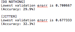
In the first part of this project, I've started out by training a baseline network consisting of 4 layers, 2 of which are convolutional layers with one at the beginning and one at the end. The last layer is a fully connected layer with each unit activated by the entire layer before it. One would imagine this to yield a solid performance, but because it is not deep enough and the input data has not been processed, we only get 29.9% accuracy using the barebones network. This is ~5% better than the 25% quoted accuracy from the project description. To maximize our performance with a network trained from scratch, we take the following approaches to improve the learnability of our training data:
- 1. Add jittering
- 2. Zero-center images
- 3. Dropout Regularization
- 4. Deeper Convolutional Networks
- 5. Batch Normalization
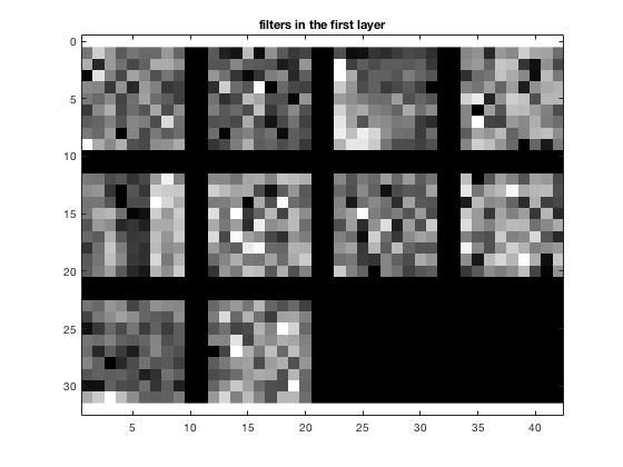
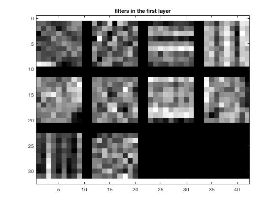
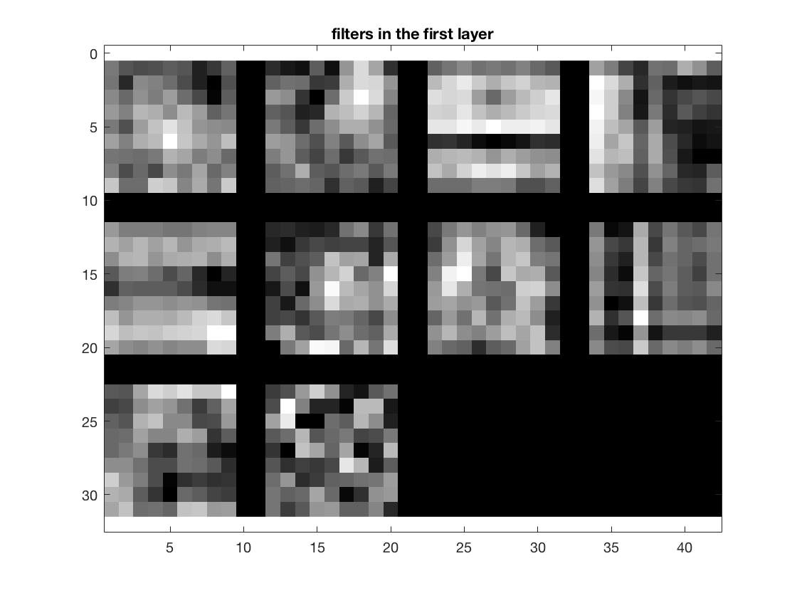
At the end of the day, I was able to bring up the recognition accuracy from 30% to about 60%, doubling the original baseline performance by making the following adjustments. We start with the baseline results visualization first.
Improvement 1: Add jittering to training data
To artificially generate more training data, we jitter the training set by randomly flipping some of the input images. Doing so moderately improved peformance, though not too much. Error rate decreases by about 3-4%.
While more elaborate forms of jittering could be utilized, after experimenting, I found it not helping very much so decided to stick with mirroring for simplicity.
Improvement 2: Zero-center the images by subtracting the mean
Using the mean2 MATLAB function I computed the mean of the image and subtracted every image from it as the chosen method to zero-center the images for better learning. The accuracy went up from 32.3% to 53.9%, showing such step to be very effective in reducing non-learnable noise. P.S. an alternative global average subtraction was later to substract average of all images from every image, which adheres to the instructions and showed slightly improved accuracy at the end of Part 1.

Improvement 3: Dropout Regularization
As its name suggests, this layer drops network connections randomly to fight the issue of overfitting. In my implementation I add a dropout layer after every convolutional layer that is not fully connected. For consistency sake when additional RELU and pooling layers are added later on, I choose to have the dropout layer added after the classic group of CONV-POOl-RELu, which seemed to also give slightly better performance (both speed and accuracy). The accuracy has now improved to 57.9%.
Improvement 4: Additional Convolutional Networks
One big success in modern neural networks is its ability to add additional layers that tend to improve overall learning accuracy with deeper networks. After experimenting with the number of convolutional layers (including RELU and POOLing) to add, as well as where to add them, and even the number of fully connected layers in the end between 1 vs. 2, I've found that the following set of network architecture and filter size + depth parameters yielded the best performance. Initially, with the following setup, I was getting 49.7% performance which was close to, but lower than the baseline shallow network's accuracy with improvements 1-3 incorporated.
49.7% Accuracy, 10-10-15 Data Depth
     layer|    0|    1|     2|     3|      4|    5|     6|     7|      8|   9|  10|     11|
      type|input| conv| mpool|  relu|dropout| conv| mpool|  relu|dropout|conv|conv|softmxl|
      name|  n/a|conv1|layer2|layer3| layer4|conv2|layer6|layer7| layer8| fc1| fc2|layer11|
----------|-----|-----|------|------|-------|-----|------|------|-------|----|----|-------|
   support|  n/a|    9|     2|     1|      1|    9|     2|     1|      1|   6|   5|      1|
  filt dim|  n/a|    1|   n/a|   n/a|    n/a|    1|   n/a|   n/a|    n/a|  10|  15|    n/a|
filt dilat|  n/a|    1|   n/a|   n/a|    n/a|    1|   n/a|   n/a|    n/a|   1|   1|    n/a|
 num filts|  n/a|   10|   n/a|   n/a|    n/a|   10|   n/a|   n/a|    n/a|  15|  15|    n/a|
    stride|  n/a|    1|     2|     1|      1|    1|     2|     1|      1|   1|   1|      1|
       pad|  n/a|    0|     0|     0|      0|    0|     0|     0|      0|   0|   0|      0|
----------|-----|-----|------|------|-------|-----|------|------|-------|----|----|-------|
   rf size|  n/a|    9|    10|    10|     10|   26|    28|    28|     28|  48|  64|     64|
 rf offset|  n/a|    5|   5.5|   5.5|    5.5| 13.5|  14.5|  14.5|   14.5|24.5|32.5|   32.5|
 rf stride|  n/a|    1|     2|     2|      2|    2|     4|     4|      4|   4|   4|      4|
----------|-----|-----|------|------|-------|-----|------|------|-------|----|----|-------|
 data size|   64|   56|    28|    28|     28|   20|    10|    10|     10|   5|   1|      1|
data depth|    1|   10|    10|    10|     10|   10|    10|    10|     10|  15|  15|      1|
  data num|   50|   50|    50|    50|     50|   50|    50|    50|     50|  50|  50|      1|
----------|-----|-----|------|------|-------|-----|------|------|-------|----|----|-------|
  data mem|800KB|  6MB|   1MB|   1MB|    1MB|781KB| 195KB| 195KB|  195KB|73KB| 3KB|     4B|
 param mem|  n/a|  3KB|    0B|    0B|     0B|  3KB|    0B|    0B|     0B|21KB|22KB|     0B|
Improvement 5: Batch Normalization
When the range of training input exceeds the range of our activation function, one common problem is that a deeper network does not learn very reasonable filters especially at the beginning. This is also attributed to the increased difficulty of gradients passing back to the first layer in a deeper architecture. One way to address this problem is to perform batch normalization on hidden layers. This allows the network to learn much quicker in the beginning since the range of the input data is normalized. The following code and ASCII diagram shows snippets of my implementation as well as the new network, which now brings the error rate down to 49.7%, giving a new high accuracy at 50.3%.
50.3% Accuracy, 32-64-15 Data Depth (referencing CNN_CIFAR example from MatConvNet)
     layer|    0|    1|     2|      3|     4|      5|    6|     7|      8|     9|     10|   11|  12|     13|
      type|input| conv| bnorm|  mpool|  relu|dropout| conv| bnorm|  mpool|  relu|dropout| conv|conv|softmxl|
      name|  n/a|conv1|layer2| layer3|layer4| layer5|conv2|layer7| layer8|layer9|layer10|conv3| fc1|layer13|
----------|-----|-----|------|-------|------|-------|-----|------|-------|------|-------|-----|----|-------|
   support|  n/a|    5|     1|      3|     1|      1|    5|     1|      3|     1|      1|    6|   6|      1|
  filt dim|  n/a|    1|   n/a|    n/a|   n/a|    n/a|   32|   n/a|    n/a|   n/a|    n/a|   10|  10|    n/a|
filt dilat|  n/a|    1|   n/a|    n/a|   n/a|    n/a|    1|   n/a|    n/a|   n/a|    n/a|    1|   1|    n/a|
 num filts|  n/a|   32|   n/a|    n/a|   n/a|    n/a|   32|   n/a|    n/a|   n/a|    n/a|   10|  15|    n/a|
    stride|  n/a|    1|     1|      2|     1|      1|    1|     1|      2|     1|      1|    1|   1|      1|
       pad|  n/a|    0|     0|0x1x0x1|     0|      0|    0|     0|0x1x0x1|     0|      0|    0|   0|      0|
----------|-----|-----|------|-------|------|-------|-----|------|-------|------|-------|-----|----|-------|
   rf size|  n/a|    5|     5|      7|     7|      7|   15|    15|     19|    19|     19|   39|  59|     59|
 rf offset|  n/a|    3|     3|      4|     4|      4|    8|     8|     10|    10|     10|   20|  30|     30|
 rf stride|  n/a|    1|     1|      2|     2|      2|    2|     2|      4|     4|      4|    4|   4|      4|
----------|-----|-----|------|-------|------|-------|-----|------|-------|------|-------|-----|----|-------|
 data size|   64|   60|    60|     30|    30|     30|   26|    26|     13|    13|     13|    8|   3|      3|
data depth|    1|   32|    32|     32|    32|     32|   32|    32|     32|    32|     32|   10|  15|      1|
  data num|   50|   50|    50|     50|    50|     50|   50|    50|     50|    50|     50|   50|  50|      1|
----------|-----|-----|------|-------|------|-------|-----|------|-------|------|-------|-----|----|-------|
  data mem|800KB| 22MB|  22MB|    5MB|   5MB|    5MB|  4MB|   4MB|    1MB|   1MB|    1MB|125KB|26KB|    36B|
 param mem|  n/a|  3KB|  512B|     0B|    0B|     0B|100KB|  512B|     0B|    0B|     0B| 14KB|21KB|     0B|
Part 1: Tuning our CNN parameters
But can we do better? Clearly, convolutional neural networks are valued for its flexibility to fine tune various learning parameters that can significantly improve performance. After tuning and tweaking with network parameters (data depth, data size and filter size at each layer) as well as the composition of network layers, the following architecture gave me ~60.7%-63% accuracy along with batch normalization included after every convolutional layer. (Jitter, Zero-centering images, dropout regularization all included)
63% Accuracy, 10-64-15 Data Depth
     layer|    0|    1|    2|    3|      4|    5|    6|    7|      8|    9|   10|   11|   12|   13|   14|     15|   16|   17|
      type|input| conv| relu|  lrn|  mpool| conv| relu|  lrn|  mpool| conv| relu| conv| relu| conv| relu|  mpool| conv| relu|
      name|  n/a|conv1|relu1|norm1|  pool1|conv2|relu2|norm2|  pool2|conv3|relu3|conv4|relu4|conv5|relu5|  pool5|  fc6|relu6|
----------|-----|-----|-----|-----|-------|-----|-----|-----|-------|-----|-----|-----|-----|-----|-----|-------|-----|-----|
   support|  n/a|   11|    1|    1|      3|    5|    1|    1|      3|    3|    1|    3|    1|    3|    1|      3|    6|    1|
  filt dim|  n/a|    3|  n/a|  n/a|    n/a|   64|  n/a|  n/a|    n/a|  256|  n/a|  256|  n/a|  256|  n/a|    n/a|  256|  n/a|
filt dilat|  n/a|    1|  n/a|  n/a|    n/a|    1|  n/a|  n/a|    n/a|    1|  n/a|    1|  n/a|    1|  n/a|    n/a|    1|  n/a|
 num filts|  n/a|   64|  n/a|  n/a|    n/a|  256|  n/a|  n/a|    n/a|  256|  n/a|  256|  n/a|  256|  n/a|    n/a| 4096|  n/a|
    stride|  n/a|    4|    1|    1|      2|    1|    1|    1|      2|    1|    1|    1|    1|    1|    1|      2|    1|    1|
       pad|  n/a|    0|    0|    0|0x1x0x1|    2|    0|    0|0x1x0x1|    1|    0|    1|    0|    1|    0|0x1x0x1|    0|    0|
----------|-----|-----|-----|-----|-------|-----|-----|-----|-------|-----|-----|-----|-----|-----|-----|-------|-----|-----|
   rf size|  n/a|   11|   11|   11|     19|   51|   51|   51|     67|   99|   99|  131|  131|  163|  163|    195|  355|  355|
 rf offset|  n/a|    6|    6|    6|     10|   10|   10|   10|     18|   18|   18|   18|   18|   18|   18|     34|  114|  114|
 rf stride|  n/a|    4|    4|    4|      8|    8|    8|    8|     16|   16|   16|   16|   16|   16|   16|     32|   32|   32|
----------|-----|-----|-----|-----|-------|-----|-----|-----|-------|-----|-----|-----|-----|-----|-----|-------|-----|-----|
 data size|  224|   54|   54|   54|     27|   27|   27|   27|     13|   13|   13|   13|   13|   13|   13|      6|    1|    1|
data depth|    3|   64|   64|   64|     64|  256|  256|  256|    256|  256|  256|  256|  256|  256|  256|    256| 4096| 4096|
  data num|   50|   50|   50|   50|     50|   50|   50|   50|     50|   50|   50|   50|   50|   50|   50|     50|   50|   50|
----------|-----|-----|-----|-----|-------|-----|-----|-----|-------|-----|-----|-----|-----|-----|-----|-------|-----|-----|
  data mem| 29MB| 36MB| 36MB| 36MB|    9MB| 36MB| 36MB| 36MB|    8MB|  8MB|  8MB|  8MB|  8MB|  8MB|  8MB|    2MB|800KB|800KB|
 param mem|  n/a| 91KB|   0B|   0B|     0B|  2MB|   0B|   0B|     0B|  2MB|   0B|  2MB|   0B|  2MB|   0B|     0B|144MB|   0B|

     layer|     18|   19|   20|     21|   22|     23|
      type|dropout| conv| relu|dropout| conv|softmxl|
      name|layer18|  fc7|relu7|layer21|  fc8|layer23|
----------|-------|-----|-----|-------|-----|-------|
   support|      1|    1|    1|      1|    1|      1|
  filt dim|    n/a| 4096|  n/a|    n/a| 4096|    n/a|
filt dilat|    n/a|    1|  n/a|    n/a|    1|    n/a|
 num filts|    n/a| 4096|  n/a|    n/a|   15|    n/a|
    stride|      1|    1|    1|      1|    1|      1|
       pad|      0|    0|    0|      0|    0|      0|
----------|-------|-----|-----|-------|-----|-------|
   rf size|    355|  355|  355|    355|  355|    355|
 rf offset|    114|  114|  114|    114|  114|    114|
 rf stride|     32|   32|   32|     32|   32|     32|
----------|-------|-----|-----|-------|-----|-------|
 data size|      1|    1|    1|      1|    1|      1|
data depth|   4096| 4096| 4096|   4096|   15|      1|
  data num|     50|   50|   50|     50|   50|      1|
----------|-------|-----|-----|-------|-----|-------|
  data mem|  800KB|800KB|800KB|  800KB|  3KB|     4B|
 param mem|     0B| 64MB|   0B|     0B|240KB|     0B|
With another set of parameter settings (see below) and the introduction of a new convolutional layer, the error rate went down even more swiftly as the number of epochs increases:
% 5x5 spatial size, 16-32-64-15 depth %
     layer|    0|    1|     2|     3|     4|    5|     6|     7|     8|      9|   10|     11|     12|     13|     14|   15|     16|
      type|input| conv| bnorm| mpool|  relu| conv| bnorm| mpool|  relu|dropout| conv|  bnorm|  mpool|   relu|dropout| conv|softmxl|
      name|  n/a|conv1|layer2|layer3|layer4|conv2|layer6|layer7|layer8| layer9|conv3|layer11|layer12|layer13|layer14|  fc1|layer16|
----------|-----|-----|------|------|------|-----|------|------|------|-------|-----|-------|-------|-------|-------|-----|-------|
   support|  n/a|    5|     1|     2|     1|    5|     1|     2|     1|      1|    5|      1|      2|      1|      1|    8|      1|
  filt dim|  n/a|    1|   n/a|   n/a|   n/a|   16|   n/a|   n/a|   n/a|    n/a|   32|    n/a|    n/a|    n/a|    n/a|   64|    n/a|
filt dilat|  n/a|    1|   n/a|   n/a|   n/a|    1|   n/a|   n/a|   n/a|    n/a|    1|    n/a|    n/a|    n/a|    n/a|    1|    n/a|
 num filts|  n/a|   16|   n/a|   n/a|   n/a|   32|   n/a|   n/a|   n/a|    n/a|   64|    n/a|    n/a|    n/a|    n/a|   15|    n/a|
    stride|  n/a|    1|     1|     2|     1|    1|     1|     2|     1|      1|    1|      1|      2|      1|      1|    1|      1|
       pad|  n/a|    2|     0|     0|     0|    2|     0|     0|     0|      0|    2|      0|      0|      0|      0|    0|      0|
----------|-----|-----|------|------|------|-----|------|------|------|-------|-----|-------|-------|-------|-------|-----|-------|
   rf size|  n/a|    5|     5|     6|     6|   14|    14|    16|    16|     16|   32|     32|     36|     36|     36|   92|     92|
 rf offset|  n/a|    1|     1|   1.5|   1.5|  1.5|   1.5|   2.5|   2.5|    2.5|  2.5|    2.5|    4.5|    4.5|    4.5| 32.5|   32.5|
 rf stride|  n/a|    1|     1|     2|     2|    2|     2|     4|     4|      4|    4|      4|      8|      8|      8|    8|      8|
----------|-----|-----|------|------|------|-----|------|------|------|-------|-----|-------|-------|-------|-------|-----|-------|
 data size|   64|   64|    64|    32|    32|   32|    32|    16|    16|     16|   16|     16|      8|      8|      8|    1|      1|
data depth|    1|   16|    16|    16|    16|   32|    32|    32|    32|     32|   64|     64|     64|     64|     64|   15|      1|
  data num|   50|   50|    50|    50|    50|   50|    50|    50|    50|     50|   50|     50|     50|     50|     50|   50|      1|
----------|-----|-----|------|------|------|-----|------|------|------|-------|-----|-------|-------|-------|-------|-----|-------|
  data mem|800KB| 12MB|  12MB|   3MB|   3MB|  6MB|   6MB|   2MB|   2MB|    2MB|  3MB|    3MB|  800KB|  800KB|  800KB|  3KB|     4B|
 param mem|  n/a|  2KB|  256B|    0B|    0B| 50KB|  512B|    0B|    0B|     0B|200KB|    1KB|     0B|     0B|     0B|240KB|     0B|
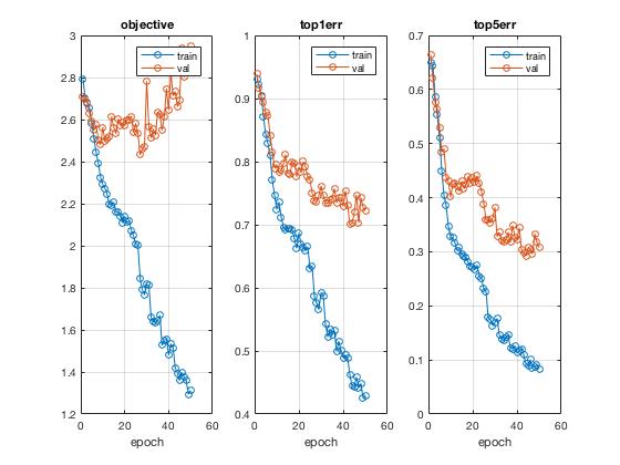
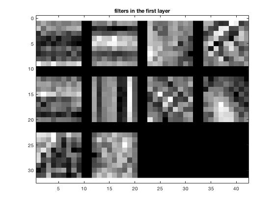
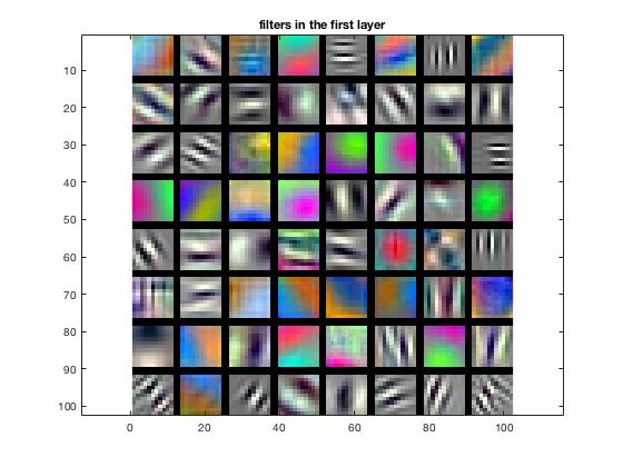
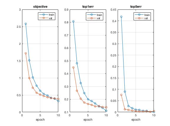
After 250 epochs, I was able to hit a record high accuracy of 68.3% with some additional creative forms of image preprocessing, including probablistic rotation, cropping and the usual flipping. On the left is a visualization of the same network trained after 40 epochs.
Part 2: Transfer Learning - Fine-tuning a pretrained VGG-F Deep Network
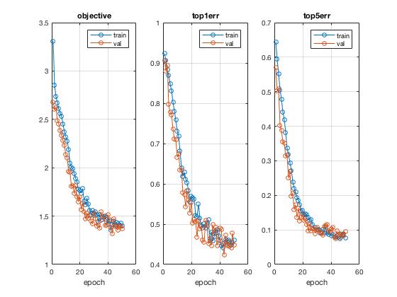
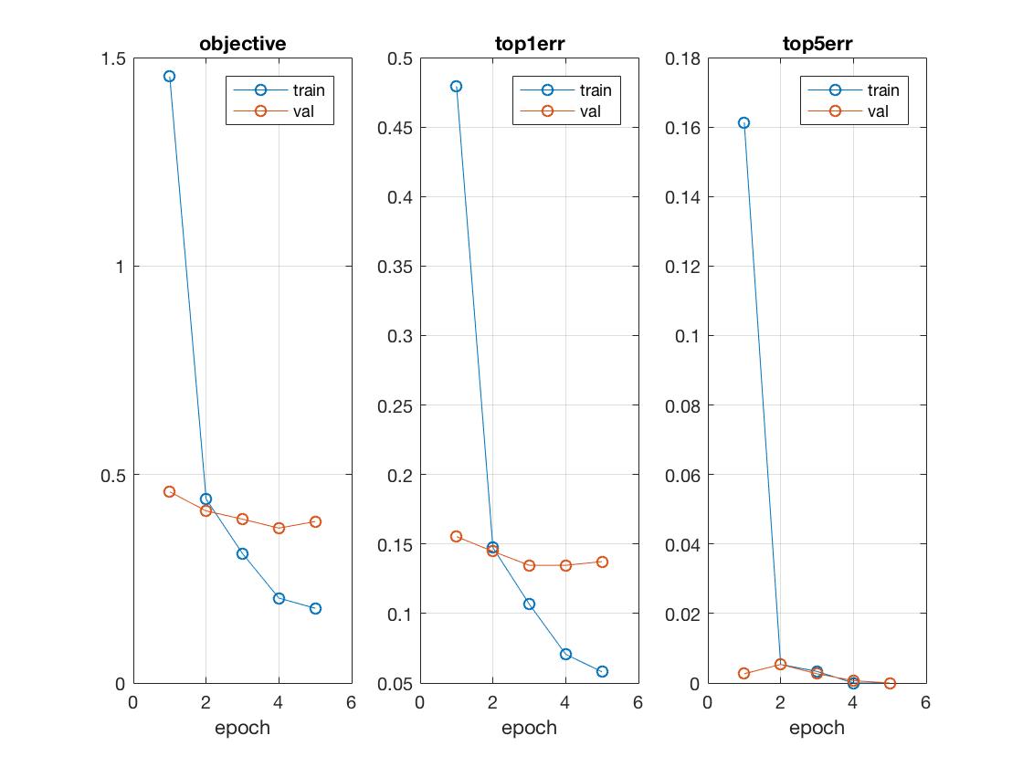
In the second part of my project, I am going to fine-tune a pretrained VGG-F network that worked really well on ImageNet for our scene classification purposes and see if it performs well on our 15 Scenes database thanks to the large amount of data it was trained on. Instead of simply extracting and subsampling existing activations from the VGG-F network, I replaced the final layer of the VGG-F network to fit it for our 15 category output as opposed to ImageNet's 1000 object categories. The weights to this new final layer re randomly initiated much like in part 1, but I also add in 2 dropout regularization layers between fc6 and fc7, as well as fc7 and fc8 (which is the final fully connected layer) to maximize performance. This approach actually dramatically reduces the training time as compared to part 1 because of the much deeper network that we have to backpropagate on. However, results are surprisingly accurate and with just 5 epochs I was able to reach 87% accuracy. I've also tried 10 epochs, which took 30-40 minutes and yielded 89.7% accuracy.
% Code snippet for replacing the final layer of the pretrained VGG-F to be retrained on 15 Scenes %
layer_count = size(net.layers,2);

net.layers{layer_count-1} = net.layers{layer_count-2};
net.layers{layer_count-2} = net.layers{layer_count-3};
net.layers{layer_count-3} = struct('type', 'dropout', 'rate', 0.5) ;

net.layers{end} = struct('type', 'dropout', 'rate', 0.5) ;
net.layers{end+1} = struct('type', 'conv', ...
                           'weights', {{f*randn(1,1,4096,15, 'single'), zeros(1, 15, 'single')}}, ...
                           'stride', 1, ...
                           'pad', 0, ...
                           'name', 'fc8') ;
net.layers{end+1} = struct('type', 'softmaxloss') ;
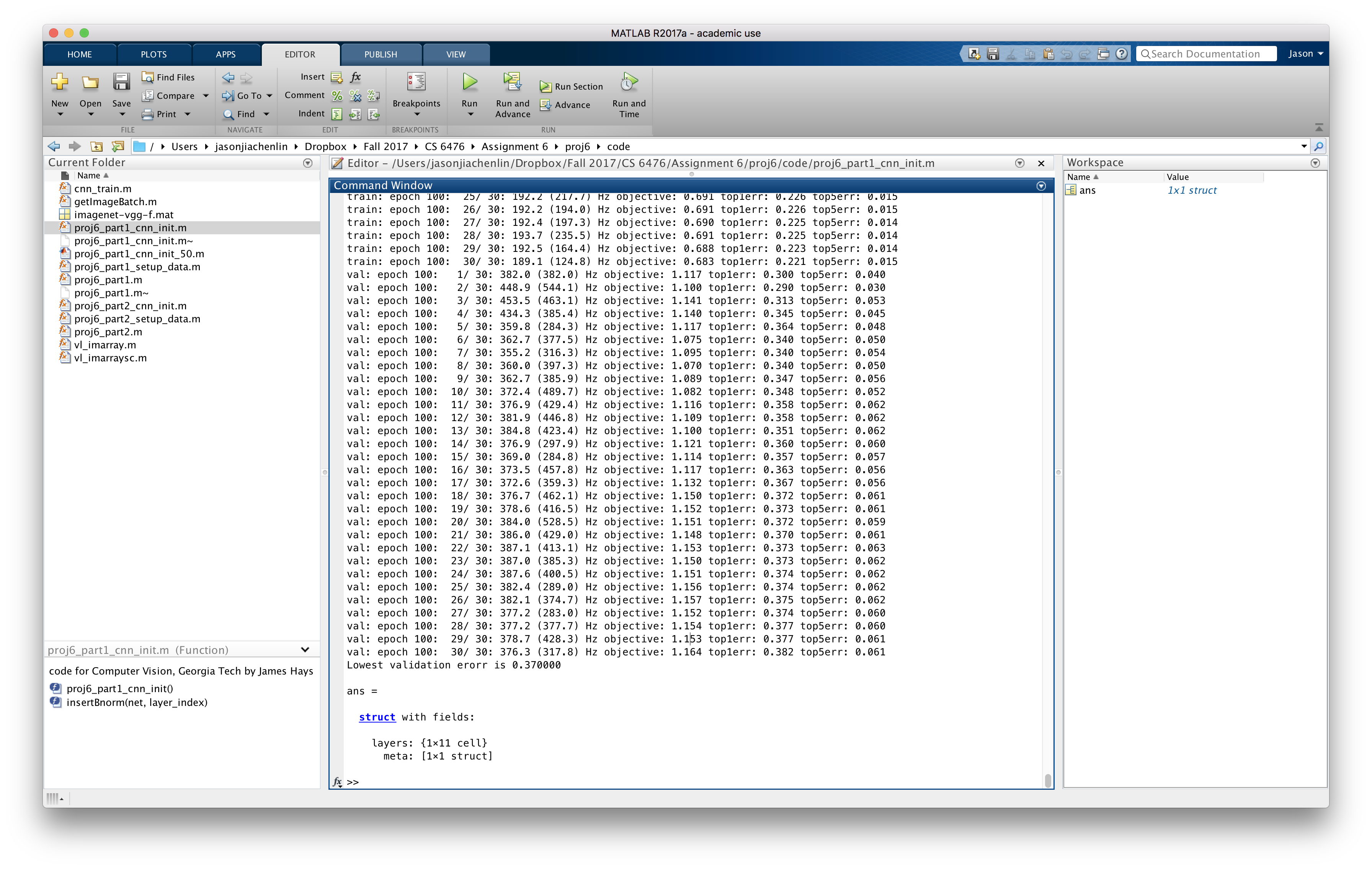
Results: 86.3% accuracy in 10 epochs, lowest top1 validation erorr = 0.137333
To ensure efficient runtime under 10 minutes, I've further fine-tuned the learning rate and maximum backpropagation depth parameters to be 0.001 and 8, respectively. By learning on stochastic gradient descent 10 times faster as well as only training the fully connected layers (fc6, fc7, fc8), I was able to cut down the number of epochs to reach an accuracy above 85% from the original 5 or 6 to 3, thereby greatly shortening the overall runtime.
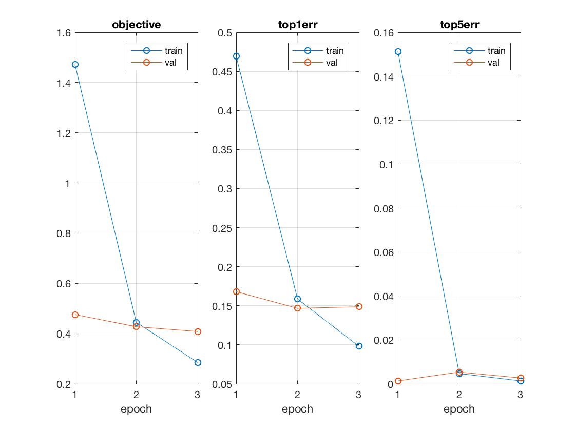
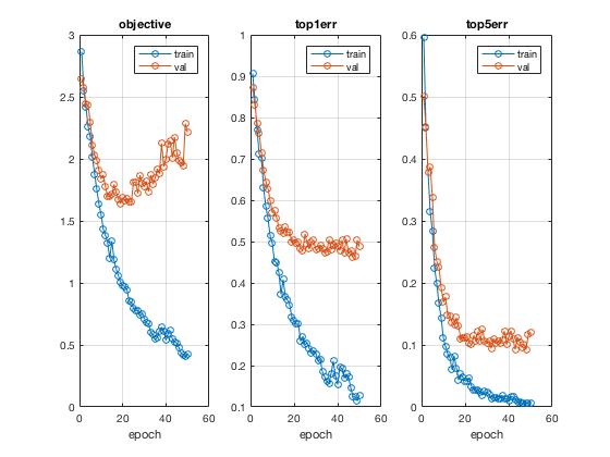
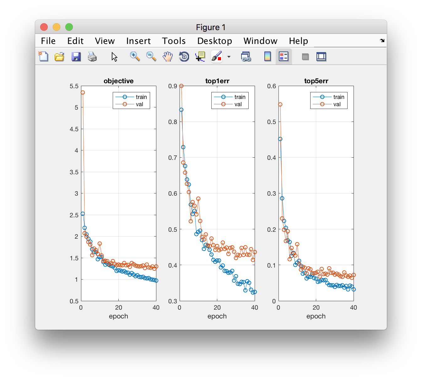
While training on the top 9 layers helped trim down the original running time by ~30%, it wasn't enough and since we really just needed to retrain the 8 fully connected layers (as shown below) that included the new layers for a sufficient degree of transfer learning, the above set of parameters seemed to give the best tradeoff balance, show in a visualization comparison between 10 epochs at 0.0001 learning rate and full backpropagation configured.
% Top 8 layers with all the fully connected layers we're retraining %
     layer|   16|   17|     18|   19|   20|     21|   22|     23|
      type| conv| relu|dropout| conv| relu|dropout| conv|softmxl|
      name|  fc6|relu6|layer18|  fc7|relu7|layer21|  fc8|layer23|
----------|-----|-----|-------|-----|-----|-------|-----|-------|
   support|    6|    1|      1|    1|    1|      1|    1|      1|
  filt dim|  256|  n/a|    n/a| 4096|  n/a|    n/a| 4096|    n/a|
filt dilat|    1|  n/a|    n/a|    1|  n/a|    n/a|    1|    n/a|
 num filts| 4096|  n/a|    n/a| 4096|  n/a|    n/a|   15|    n/a|
    stride|    1|    1|      1|    1|    1|      1|    1|      1|
       pad|    0|    0|      0|    0|    0|      0|    0|      0|
----------|-----|-----|-------|-----|-----|-------|-----|-------|
   rf size|  355|  355|    355|  355|  355|    355|  355|    355|
 rf offset|  114|  144|    114|  114|  114|    114|  114|    114|
 rf stride|   32|   32|     32|   32|   32|     32|   32|     32|
----------|-----|-----|-------|-----|-----|-------|-----|-------|
 data size|    1|    1|      1|    1|    1|      1|    1|      1|
data depth| 4096| 4096|   4096| 4096| 4096|   4096|   15|      1|
  data num|   50|   50|     50|   50|   50|     50|   50|      1|
----------|-----|-----|-------|-----|-----|-------|-----|-------|
  data mem|800KB|800KB|  800KB|800KB|800KB|  800KB|  3KB|     4B|
 param mem|144MB|   0B|     0B| 64MB|   0B|     0B|240KB|     0B|
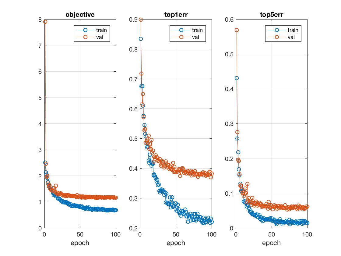
Training on the top 8 layers for 30 epochs gave very promising results, nearing 90% accuracy. This can take a while though. 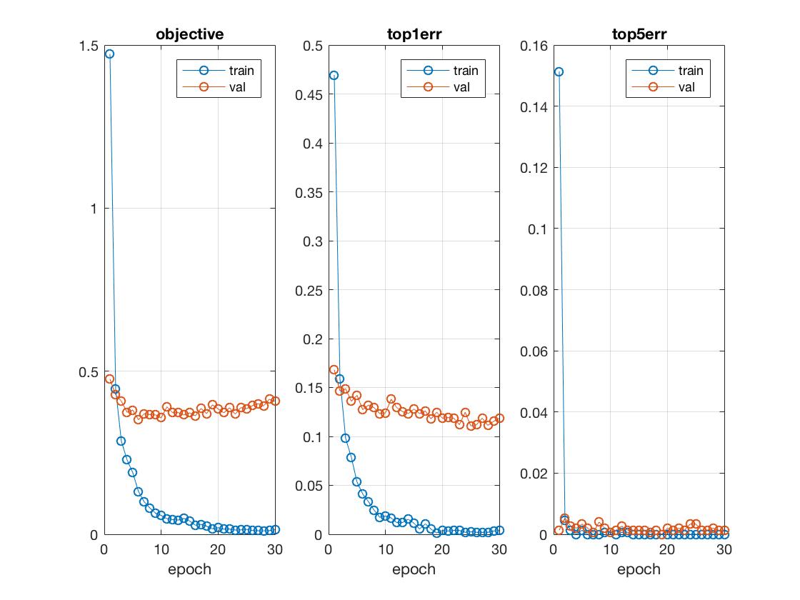 Since the error trend was still downward by 30th epoch, had I ran for more epochs the accuracy is likely to break 90%. I've tried running for 50 epochs, but due to the recursive nature of the MATLAB Java program, I ran out of disk memory at around 35 epochs.
Conclusion
Overall, the findings from this project is promising: that with deeper networks, we can expect much better scene recognition performance given the right convolutional architecture and equally importantly a well fine-tuned set of neural network and testing parameters. In general though, the quality and learnability of training data can also improve the network observably, especially if we have a shallow network like the one we trained from scratch in part 1.